An Analysis on Technical Efficiency in Post reform China

Munich Personal RePEc Archive

An Analysis on Technical Efficiency in

Post-reform China

Zhou, Xianbo and Li, Kui-Wai and Li, Qin

2010

Online at

https://mpra.ub.uni-muenchen.de/41034/

China Economic Review

, 22 (3) September, 2011: 357-372

An Analysis on Technical Efficiency in Post-reform China

Xianbo Zhoua，Kui-Wai Lib†and Qin Lia

a

Lingnan College, Sun Yat-Sen University, China

b

Department of Economics and Finance, City University of Hong Kong

Abstract:

This paper employs a fully nonparametric stochastic frontier model with time and

individual effects to study technical efficiency in China’s post-reform economy. The

panel data cover China’s thirty provinces for the period of 1985-2008. The empirical

results show that the average output elasticity of labor is larger than the other two inputs of capital and human capital. Based on the specified inefficiency Tobit model, the factor analysis on technical efficiency shows that the time effects of technical efficiency in

China’s post-reform economy are significantly contingent on the factors. There exists

significant regional differences in technical efficiency in China’s economic development,

and a number of policy implications can be drawn.

Key words: Fully nonparametric stochastic frontier; time effects and individual effects; time variant; technical efficiency; Tobit model.

JEL Classifications: C52, D24, O47 _____

† _{Corresponding author: Kui-Wai Li, City University of Hong Kong, Tel.: 852 34428805;}

Fax.: 852 34420195; E-mail: [email protected].

Acknowledgement: The authors are indebted to the invaluable comments from the referees and would like to express their gratitude for the various research funding

supports. Zhou’s research was supported by the National Natural Science Foundation of

China (Grant 70971143), and Li’s research funding was supported by the City

University of Hong Kong under two Strategic Research Grants (Numbers 7001907 and

7002175).Research assistance from Liang Wang, Helen H. K. Lam, Pang Yu and Lan

1. Introduction

The discussion on the sustainability of economic growth in China’s post-reform

economy has led to studies on China’s productivity, using either growth accounting or

stochastic frontier analysis (SFA) (Chen et al., 2009; Chen et al., 2008; Wu, 2000, 2003,

2004; Hu and Khan, 1997; Woo, 1998; Mao and Koo, 1997; Borenstein and Ostry, 1996;

Yang and Lahr, 2010). For example, the studies by Chow and Li (2002) and Li (2003)

used investment figures to construct capital stock to estimate China’s national total

factor productivity (TFP) growth rates have been extended by Liu and Li (2006) and Li

(2009) who incorporated the human capital variable and alternative investment data to

examine both national and provincial TFP growth rates. Similar studies by Wang and

Yao (2003) have examined the sources of China’s economic growth, while Swamy

(2003), Motohashi (2007) and Bosworth and Collins (2008) have compared China’s

TFP with other world economies.

In studying the technical change in the United States, Solow (1957) differentiated

the movement along the production function caused by input growth from shift in the

production function caused by technical progress. Both Bauer (1990) and Kumbhakar

and Lovell (2000) have shown that TFP growth composes of technical progress,

technical efficiency change and a scale economies effect. In theory, technical progress is

an outward shift of the production frontier and technical efficiency change shows the

movement from a position within towards a position on the production frontier, while

the scale economies effect reflects an increase in return to scale.

Other studies have elaborated and extended China’s post-reform economic

productivity to efficiency analysis by using the Malmquist productivity index (MPI) and

data envelop analysis (DEA) (Wu, 1995, 2008). The MPI that decomposes productivity

into efficiency and technological change has also been applied in Ma et al. (2002) and

Movshuk (2004). Studies on the productivity and efficiency performance of individual

industries in China have been conducted by Jefferson (1990) and Mu and Lee (2005),

while Yao et al. (2007) and Sun et al. (1999) agreed that SFA and DEA are the more

effective approach to measure the technical efficiency of industries. The SFA used in

function and technical efficiency performance (Huang and Kalirajan, 1998; Kalirajan et

al., 1996; Brummer et al., 2006; Hu and McAleer, 2005; Tong, 1999; Wu 2000, 2003;

Fu, 2005).

Nonetheless, studies on China’s post-reform economy have provided a continued

debate on whether technical progress or technical efficiency is the more important

contributing factor to China’s TFP growth (Wu, 2000; Li and Liu, 2011). After more

than three decades of economic reform since 1978, it would be useful to examine if

technical efficiency has become an important factor in China’s growth. In addition, an

objective measure on the technical efficiency among China’s provinces is crucial. Given

the extraordinary nature, the heterogeneity of development in various regions and

different time periods, a flexible stochastic frontier model can be used to study technical

efficiency in the post-reform China’s economy.

Empirical studies using the conventional stochastic frontier analysis on panel data

models often implicitly impose a restriction that information differences have no effect

on the way risk-neutral decision makers utilize the same input bundle (Christopher et al.,

2010). The result is that informational differences are mistaken for differences in

technical efficiency. The two specific effects that reflect information differences are the

individual effects and the time effects. They are usually specified in stochastic frontier

models in the manner that individual effects are time-invariant and do not interact with

time effects, often in linearity or in parametric forms. However, when the individuals in

the sample differ in technology and efficiency with differenced information, especially

when such heterogeneity changes with time, the linear or parametric specification

cannot fully describe the heterogeneity in the production function and may induce a bias

in the measurement of technical efficiency. Conventional methods (either DEA or SFA)

attribute the model misspecification errors to inefficiency (Fu, 2005; Balaguer-Coll et

al., 2007; Grösche, 2009; Joseph et al., 2010; Battese and Coelli, 1992, 1995;

Kumbhakar and Lovell, 2000; Wu 2003). Researchers have relaxed distributional

assumptions in the error component and parametric assumptions in SFA to achieve a

more reliable measurement of technical efficiency (Greene, 2005; Kneip and Simar,

The data set used in this study contains the thirty provinces in China for the period

from 1985 to 2008. One can note that China during the sample period has experienced a

systemic transition with heterogeneity of provinces and development periods. The

regional effects and time effects should be given sufficient attention in measuring the

technical efficiency of the economy. This paper provides a time-variant estimation of

technical efficiency in China’s post-reform economy by specifying and estimating a

fully nonparametric stochastic frontier model with nonparametric individual and time

effects (Henderson and Simar, 2005). A factor analysis on technical efficiency by using

the Tobit regression will also be conducted.

Section 2 specifies the nonparametric model and presents the estimation method.

Data and variables specification are illustrated in Section 3. Section 4 presents the

empirical results of the frontier model and the measurement of the technical efficiency.

Section 5 provides the specification test to show the suitability of the nonparametric

model. Section 6 provides a factor analysis on the technical efficiency based on the

Tobit estimation. Section 7 concludes the paper.

2．Fully Nonparametric Model Specification

The studies in Gong and Sickles (1992) and Christopher et al. (2010) show that the

estimates of technical efficiency for the parametric panel data frontier model can be

improved when the production function model is closer to the true underlying

technology. In practice, the data generating process is unknown and so are the stochastic

factors in the economic data. Hence a flexible model specification will give a more

reliable result on frontier and efficiency estimates. In our sample period, production

technology and efficiency in China has experienced uneven development among

different provinces. A fully nonparametric stochastic model can thus give reliable

technical efficiency estimates. We specify the nonparametric stochastic frontier model

as follows:

( , , ) , 1, 2, , ; 1, 2, ,

it it it

where yit is the logarithm of real gross regional product (RGRP) for province i in

year t; xit is the vector of the logarithm of the three inputs: capital (K), labor (L) and

human capital (HC); f x i t( , , ) is the production function which is allowed to vary over

each province and time period, and is nonparametric with input variables x, individual

effects and time effects; uit is the error term independent of xit. As we know, human

capital may have an impact on production through both direct and indirect channels

(Barro and Sala-i-Martin, 1999; Benhabib and Spiegel, 2005; Vandenbussche et al.,

2006). Equally, the human capital embodied in the labor force can exert a direct and an

indirect influence on aggregate production through technological innovation, imitation

and adoption. Given that the impact channels are uncertain, it would be appropriate to

allow human capital to enter the production function and interact with capital and labor

inputs, individual and time effects in a nonparametric manner.

Model (1) can be estimated using the approach in Henderson and Simar (2005).

Denote ( , , )x i t as the first derivative of f x i t( , , ) with respect to x. By the Taylor

expansion,

( , , ) ( ) ( , , ) (| |)

it it it it

y  f x i t  x x  x i t o x x u , (2)

where o x(| itx|) is the higher-order term of |xitx|. Since we apply the local linear

estimation, and the higher-order term is o h(| c|) as the bandwidth hc of the

continuous variable tends to zero, and hence the higher-order term can be merged into

the error term and does not affect the consistency of the nonparametric function. Note

that the frontier function includes unordered categorical variable i and ordered

categorical variable t. To smooth them, the following kernel function is applied:

( , , )

ijts c u o

K h h h 









q

r js r cr u ij o ts r k x x h l l



where ( )k  is the kernel for continuous input variables; lu ij, and lo ts, are the kernels

, 1, , , u ij u j i l

h j i

 

  _

 and ,

 

1, , , . s t o ts o s t l

h  s t

 

 



 .

As hu 0, lu ij, 1{ji} is the indictor function of province i, implying that only the

data of province i are used in the estimation; as hu 1, lu ij, 1, the product kernel is

unrelated to province i, implying that individual effects have been smoothed out. Now

u

h is allowed to change continuously, and is combined with the above two special

cases and plays a role in the smoothness of individual effects. In the similar way, ho

plays a role in the smoothness of time effects. We call hc (hc1, ,hcq), ,h hu o the

smoothers or bandwidths for continuous variables, individual variable, and time

variable, respectively. LetXjs (1,xjsx). From (2),

' '

( , , )x i t ( ( , , ), ( , , ) )f x i t x i t

  

can be estimated by

1

' '

1 1 1 1

ˆ_{( , , )} n T _{ijts( , , )c u o js js} n T _{ijts( , , )c u o js js}

j s j s

x i t K h h h X X K h h h X y





   

   

    







The optimal bandwidth ( , , )h h hc u o can be determined by the least squares cross

validation (LSCV) approach:

0

(hc, , )h hu o ＝

2

0 _{1 1} ˆ

arg minCV b( c, , )b bu o 

 

Here fˆi( , , )x i tit is the leave-one-out estimator of f x i t( , , )it with bandwidths hc,bu

and bo, where b0c,h hu, o are positive constants,

1/(4 ) 0 ( )( )

q c c

h b std x nT   , and std x( )

denotes the sample standard deviation vector.

Following Henderson and Simar (2005), the estimate of technical efficiency for

province i in time period t is defined as

ˆ

exp ( , , )

it _it

TE f x i t

1, ,

ˆ

max ( , , )it

j nf x j t . (5)

Essentially the measure of technical efficiency compares the difference between the

actual (estimated) outputs of province i and the maximum potential output produced by

any other province in the sample for the same time period.

specifications of semiparametric and parametric models for comparison. The purpose is

to know what will happen to the estimates when restrictive specifications on the

technology are estimated. The two special cases are restricted forms of Model (1) with

time-invariant production functions instead of time-variant ones. In the semiparametric

case, the specification is

( ) , 1, 2, , ; 1, 2, ,

it it i it

y  f x    u  i n t T (6)

where f( ) is a nonparametric function of the inputs to be estimated, which is an

averaged and time-invariant production function, and the fixed effects  i  ui enter

the model in a linear and additive form which is also time-invariant. The function f( )

can be estimated, denoted as fˆ( ) , by the locally linear nonparametric kernel methods

(Li and Racine, 2007). The parametric case is a particular case of the semiparametric

form with '

( )it it

f x x  :

'

, 1 , 2 , , ; 1 , 2

i t i t i i t

y  x  u  i  n t (7)

The parameter, denoted asˆ, can be estimated by the conventional within-estimator

for panel data models with fixed effects. The technical efficiency for province i is

defined as (Kneip and Simar, 1996)

ˆ

exp )

i _i

TE u , (8)

where in a normalization form uˆi 

i ˆ

maxi ˆi, ˆi ₁( ˆ( )) / T

it it t y f x T





semiparametric case, and ˆi

' 1( ˆ) /

T

it it t y x  T





apply specification tests only to the most suitable model in our empirical study.

3. Data and Variables

Despite the debate on the accuracy of macroeconomic data and the lack of a

reliable alternative set of economic data in post-reform China, empirical studies have

Holz, 2006; Chow 2006).1

Other than accuracy, critics have noted a number of

problems in China’s macroeconomic data. One concern is the transformation from the

Soviet material product system (MPS) to the system of national accounts (SNA) as the

former does not value “non-market” and “non-materials” output and services and

another concern is the deficiency in China’s national account and statistical practice

(Maddison and Wu, 2008; Wu, 2000, 2003).2 Others have concentrated on the

estimation of the capital stock series, and that such detailed measures as the scrap rate

and depreciation rate of the same capital equipment at different years are absent (Wu,

2007; Holz, 2006). A number of empirical studies agree that problems in the time series

data may cancel out each other and that China’s statistical reporting system and data

reliability have improved over the years (Chow and Li, 2002; Li, 2003, 2009; Szirmai et

al., 2005).

The data for China’s thirty provinces and the construction of key variables used in

this paper are elaborated in the Appendix. The thirty provinces that include the four

autonomy areas and three municipalities under direct central administration are

geographically divided into four regions. The Southern region composes of nine

southern provinces, commonly known as the Pearl River Delta provinces of Fujian,

Guangdong, Guangxi, Hainan, Jiangxi, Hunan, Sichuan (including Chongqing since

1997), Guizhou and Yunnan. The Eastern region consists of twelve provinces, including

mainly provinces in the Yellow River and Yangtze River Delta regions of Beijing,

Tianjin, Hebei, Shanghai, Jiangsu, Zhejiang, Shandong, Anhui, Henan, Hubei, Shanxi

and Gansu. The Western region refers to the remote provinces of Inner Mongolia, Tibet,

Shaanxi, Qinghai, Ningxia, and Xinjiang. The remaining three provinces in

Northeastern region are Jilin, Heilongjiang and Liaoning, which consist of the

traditional state-owned heavy industries. These four sub-regions in China are chosen in

our study to reflect the geographical strength and economic growth concentration.

China’s national and regional output figures can be obtained, respectively, from the

1 _{China’s GDP has been revised upwards by US$300 billion in December 2005.}

South China Morning Post, December 13 and 21, 2005, and January 13, 2006.

2 _{For example, China’s National Bureau of Statistics (NBS) reported in December 2004 that by incorporating}

Statistical Yearbook of China and the various provincial statistical yearbooks. Scholars

have used national income and sector output to construct China’s physical capital stock

(Jefferson et al., 1996; Wu, 1995, 2008). One reliable method shown in Chow and Li

(2002) and Li (2003) is Chow’s (1993) estimation of China’s 1952 physical capital

stock. Based on the “accumulation” figures available up to 1978 in the official statistics

and the additional comparable net investment and provincial depreciation figures since

1978, the construction of China’s national and provincial physical capital stock series

have been extended to 1998. While Li (2009) has repeated the construction exercise and

extended the data to 2006, the analysis in this paper adopts the same steps and extends

China’s provincial physical capital stock to 2008. The data of the labor inputs are the

total employed persons (in ten thousand persons) obtained from the Statistical Yearbook

of China.

Human capital has been considered as an endogenous growth variable (Romer,

1990; Tamura, 2002, 2006; Turner et al., 2008). Similarly, there have been alternative

methods in constructing human capital (Gemmell, 1996; Zhang et al., 2005; Chi, 2008).

The inventory approach used in Wang and Yao (2003) measures China’s human capital

stock per capita in average years of schoolingfor the period 1984-2000. In Liu and Li

(2006) and Li et al. (2009), the years of schooling are divided into six levels (primary

education, junior secondary, senior secondary, vocational secondary, specialized

secondary and higher education). The inventory-based construction of the human capital

stock has been adjusted by inter-provincial migration and mortality rates from the

estimated census data. Since 2004, the six levels of schooling have been reclassified

into four levels of primary education, junior middle education (including regular junior

middle and vocational junior middle education), senior middle education (including

regular senior middle, vocational middle and specialized secondary), and higher

education. Following Li (2009, Appendix), standard assumptions on the transition

between different classifications are used so that national and regional human capital

stocks per capita adjusted by employment figures can be updated to 2008 (see

Appendix). Li et al. (2009, Table 3) reports that the estimation on China’s human capital

study has shown that China’s human capital is lower than that of other Asian economies.

In order to eliminate the size effect of the provinces that may affect the measure of

technical efficiency, we include in the denominator of each province’s real gross

regional product (RGRP), physical capital stock and labor inputs the province’s total

population. Kneip and Simar (1996) and Henderson and Simar (2005) have also made

such an adjustment in their frontier models to measure technical efficiency. Table 1

provides the simple statistics for the data of the four variables. The coefficients of

variation in the last column of Table 1 show that RGRP and physical capital stock have

much larger degrees of variation than the other two variables in our sample.

Table 1 Summary Statistics of the Data (30 provinces: 1985-2008)

average min max stdev coefficient of variation

RGRP/Population 2581.71 326.26 26576.64 2936.55 114%

Capital/ Population 9219.06 848.10 86385.38 11103.96 120%

Labor/ Population 0.51 0.36 0.82 0.07 15%

Human Capital 5.45 0.74 10.88 1.90 35%

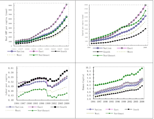
Figure 1 reports the dynamic average performances of the four variables. One

general observation is that these variables show obvious time trends in the sample

period, especially since the late 1990s. The labor per capita variable has shown a clear

structural break. The Eastern region has the highest average RGRP per capita. The

Northeastern region has a similar level of RGRP per capita to the national average,

whereas the Western and Southern regions have a lower level than the national average.

Although the Northeastern region has the highest level of physical capital and human

capital per capita, it has the lowest labor per capita. The differences in RGDP, level of

physical capital stock and human capital per capita across provinces and regions show

clearly that there are great variations in the development paths among the provinces in

China’s post-reform economy. The statistical evidences shown in Table 1 and Figure 1

hint that a flexible time-variant stochastic econometric model with individual effects

and time effects may be required in order to estimate a reliable measure of technical

0 1000 2000 3000 4000 5000 6000 7000 8000 9000

1984 1987 1990 1993 1996 1999 2002 2005 2008

Real GRP per capita (yuan)

Nation East South

West Northeast 0 3000 6000 9000 12000 15000 18000 21000 24000 27000 30000

1984 1987 1990 1993 1996 1999 2002 2005 2008

Capital per capita (yuan)

Nation East South West Northeast 0.40 0.43 0.46 0.49 0.52 0.55 0.58 0.61

1984 1987 1990 1993 1996 1999 2002 2005 2008

Labor per capita

Nation East South

West Northeast 3.0 3.8 4.6 5.4 6.2 7.0 7.8 8.6 9.4 10.2

1984 1987 1990 1993 1996 1999 2002 2005 2008

H u m a n C a p i t a l

Nation East South West Northeast

Figure 1 Dynamics of China’s Average Real GDP or GRP per capita (1985-2008)

4. Estimation Results

In order to provide a comparison with the estimation of the nonparametric

specification indicated in Model (1), we also specify two other restricted versions with

time-invariant specification, namely, the semiparametric Model (6) and the parametric

Model (7). All the variables are expressed in logarithms. The variables are adjusted for

the time trend effect in the two restricted models, but not in the nonparametric Model (1)

because the time effect has already been picked up by the categorical variable. This

time-effect adjustment for dependent and independent variables in the time-invariant

technical efficiency for the two restricted versions is calculated from Model (8).

In the nonparametric estimation of Model (1) and Model (6), we select the

fourth-order Gaussian kernel function



 



( ) 1.5 0.5 exp / 2 / 2

k u   u u  to

alleviate the curse of dimensionality since the dimension of the input variables is three.

By using the least squares cross validation (LSCV) approach shown in (4), the optimal

bandwidths of the three continuous input variables are 0.492, 0.072 and 0.217, and the

optimal bandwidths of categorical variable i and ordered categorical variable t are

0.153 and 1.035, respectively, for the estimation of Model (1).3 The LSCV optimal

bandwidths of the three continuous input variables for the local linear nonparametric

estimation of the semiparametric Model (6) are 0.051, 0.046 and 0.041.4

We use R2, the squared correlation coefficient between the dependent variable and

the fitted value, to measure the goodness-of-fit for the estimated model. The R2 values

for the estimation of the three models are shown in the last column of Table 2, and the

values given by parametric and semiparametric models are 0.38 and 0.48, respectively.

The nonparametric estimation gives a large goodness-of-fit measure with R2 = 0.98.5

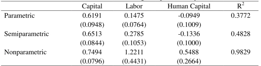
Table 2 Estimation of Average Output Elasticity

Capital Labor Human Capital R2

Parametric 0.6191 0.1475 -0.0949 0.3772

(0.0948) (0.0764) (0.1009)

Semiparametric 0.6513 0.2785 -0.1336 0.4828

(0.0844) (0.1053) (0.1000)

Nonparametric 0.7494 1.2211 0.5488 0.9829

(0.0796) (0.4431) (0.2664)

Note: The values in parenthesis are the bootstrapped standard errors of the estimates. The replications are 400.

3 _{In order to examine the effect of the kernel selection on the estimation results, we also apply the second-order and}

the sixth-order Gaussian kernel for the nonparametric estimation. It is found that the results are quite similar. Hence we only report the results from the fourth-order Gaussian kernel.

4 _{The optimal bandwidths chosen in the nonparametric estimation of the semiparametric model (6) are much smaller}

than those in the nonparametric estimation of the nonparametric model (1). This is due to the fact that the variables have been adjusted for the time effect in the semiparametric model (6) but not in the nonparametric model (1). However, the categorical variable t in nonparametric model (1) picks up the time effect with an optimal bandwidth of 1.035.

5 _{Note that the R}2 _{from the nonparametric estimation is not suitably compared with the R}2_{sfrom the parametric and}

Table 2 shows the sample average of the output elasticity estimates of the three

inputs in the three specification models and their corresponding bootstrapped standard

errors. In the parametric and semiparametric models, the coefficient estimates of capital

and labor are positive and significant, while the coefficient estimates of human capital,

though insignificant, are negative and unexpected. However, the elasticity estimates of

the three inputs in the nonparametric model are positive and significant, which can

provide expected and meaningful economic explanation. When compared to other

studies, for example, by Young (2003) and Li (2009) who do not estimate the output

elasticity of inputs by using per capita output and inputs, our finding shown in Table 2 is

that the output elasticity of labor, instead of the elasticity of capital, is the largest of the

three inputs.

Table 3 presents the estimates of the yearly average technical efficiency of the 30

provinces. The average time-invariant technical efficiency results are calculated

according to the parametric Model (7) and semiparametric Model (6) using formula (8),

while the average time-variant technical efficiency results are calculated according to

the nonparametric Model (1) using formula (5).

Table 3 shows a large discrepancy in the ranking of provinces between the

semiparametric and parametric models for a majority of provinces. Only the three

provinces of Beijing, Heilongjiang and Jiangxi are ranked in almost the same order

between the two estimates. Such a result, along with the weak goodness of fit and the

meaningless and insignificant coefficient estimates of human capital, suggests that the

time-invariant assumption shown by the linear parametric and semiparametric models

may be incorrect. The less restrictive nonparametric time-variant model can correctly be

used to calculate the time-variant technical efficiency. Indeed, many of the rankings in

the nonparametric model differ significantly from those in the parametric and

semiparametric models.

Province Parametric Semiparametric Nonparametric DEA

TE rank TE rank TE rank TE rank

Beijing 0.2309 29 0.9901 28 0.7988 27 0.6941 17

Tianjin 0.2840 27 0.9905 24 0.8924 21 0.8474 8

Heibei 0.7621 8 0.9980 3 0.9794 9 0.9252 5

Shanxi 0.6185 16 0.9903 25 0.8478 25 0.6018 24

Inner Mongolia 0.6267 13 0.9923 17 0.9504 15 0.7031 16

Liaoning 0.2576 28 0.9922 18 0.6885 30 0.6123 23

Jilin 0.6204 15 0.9864 30 0.9153 19 0.7496 15

Heilongjiang 0.6294 12 0.9930 12 1.0000 1 0.8059 11

Shanghai 0.1839 30 0.9931 11 0.9575 14 1.0000 1

Jiangsu 0.4151 25 0.9917 19 0.9598 13 1.0000 2

Zhejiang 0.4270 24 0.9952 6 0.9954 6 0.8626 7

Anhui 0.7821 5 0.9934 9 0.9924 8 0.7610 14

Fujian 0.6014 17 1.0000 1 1.0000 2 0.8423 9

Jiangxi 0.7683 7 0.9935 7 0.9682 11 0.7624 13

Shandong 0.5856 18 0.9934 10 0.9324 16 0.8685 6

Henan 0.7571 9 0.9915 20 0.8625 24 0.6927 19

Hubei 0.6775 11 0.9929 14 0.9997 3 0.8095 10

Hunan 0.8760 3 0.9902 27 0.9945 7 0.7865 12

Guangdong 0.5441 22 0.9955 5 0.9784 10 0.9967 3

Guangxi 1.0000 1 0.9929 15 0.9032 20 0.6935 18

Hainan 0.5446 20 0.9957 4 0.8680 23 0.6185 22

Sichuan 0.7820 6 0.9912 22 0.9976 4 0.9911 4

Guizhou 0.9786 2 0.9890 29 0.9154 18 0.5914 25

Yunnan 0.8543 4 0.9924 16 0.9671 12 0.6653 20

Tibet 0.3752 26 0.9999 2 0.9967 5 0.3878 30

Shaanxi 0.6227 14 0.9915 21 0.8404 26 0.5638 27

Gansu 0.6838 10 0.9903 26 0.9310 17 0.6497 21

Qinghai 0.5445 21 0.9912 23 0.7565 28 0.4713 28

Ningxia 0.4996 23 0.9930 13 0.7558 29 0.4506 29

Xinjiang 0.5496 19 0.9935 8 0.8740 22 0.5793 26

The nonparametric time-variant model estimation provides more information on the

provinces and time dependent structure of the efficiencies. Appendix Table A1 reports

the yearly technical efficiency scores of all provinces based on the nonparametric Model

(1) and the formula (5). The scores show that the two provinces of Heilongjiang and

Fujian are technically efficient in all years during the sample period. A total of thirteen

provinces (Beijing, Shanxi, Liaoning, Jilin, Henan, Guangxi, Hainan, Guizhou, Shaanxi,

Gansu, Qinghai, Ningxia, and Xinjiang) are not technically efficient in any year; the

ranked 27th in technical efficiency and is less efficient than many other provinces.

It can be calculated from Appendix Table A1 that 29.7 percent of observations (720

observations from 30 provinces in 24 sample years) have attained technical efficiency.

The coefficient of variation for technical efficiency estimates is 10.6 percent, which

shows that the difference of technical efficiency among the provinces should not be

ignored. Such a finding is not available from the time-invariant parametric or

semiparametric models.

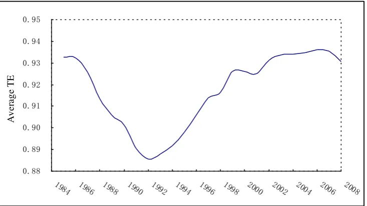
Figure 2 presents the dynamics of the average technical efficiency for the 30

provinces in the sample period. Economic liberalization in the early years of economic

reform and openness has probably led to the initial increase in technical efficiency. The

initial increase in technical efficiency, however, was not sustainable. The technical

efficiency declined rapidly to the lowest level in 1992 before it bounced back and

reached new peaks in 1998 and 2006.

0.88 0.89 0.90 0.91 0.92 0.93 0.94 0.95

198₄ 198₆ 198₈ 199₀ 199₂ 199₄ 199₆ 199₈ 200₀ 200₂ 200₄ 200₆ 200₈

A

v

er

ag

e

TE

Figure 2 The Dynamics of Technical Efficiency

Figure 3 shows the regional variation in the dynamics of average technical

efficiency. At the national level, and despite the marginal decline between 1985 and

1992, the overall trend has been a gradual increase in technical efficiency. Both the

Eastern and Southern regions have shown a better performance than the national

efficiency than the national average. Provinces in the Northeastern region have shown a

lowest level of technical efficiency before 1994, but since then, it has overtaken the

Western region. Although there has been much attention and emphasis on the economic

development in the Western region, its technical efficiency has remained backward,

probably due to the faster economic development in the Eastern and Southern regions

that had made the interior regions unattractive. Technical efficiency tends to be higher

than the national average in the Eastern and Southern regions, which historically have

been the most developed regions in China.

0.76 0.79 0.82 0.85 0.88 0.91 0.94 0.97 1.00

198₄ 198₆ 198₈ 199₀ 199₂ 199₄ 199₆ 199₈ 200₀ 200₂ 200₄ 200₆ 200₈

Average TE

Nation East South West Northeast

Figure 3 The Dynamics of Average National and Regional Technical Efficiency

5. Model Specification Test and Discussion

The semiparametric Model (6) and the linear parametric Model (7) assume

time-invariant specifications in the estimation of technical efficiency, while the

nonparametric Model (1) allows a flexible production specification with time-variant

production technology. We have shown that the efficiency rankings among provinces in

China differ greatly in the different approaches used to measure technical efficiency,

and that the nonparametric specification is most suited to our sample. For a rigid

This section presents two tests for model specification. The first test is to choose

between (6) and (7). The null hypothesis is linear parametric Model (7) and the

alternative is semiparametric Model (6). The second test is to choose between (1) and

(6). The null hypothesis is semiparametric Model (6) and the alternative is

nonparametric Model (1). We apply the test approach in Henderson et al. (2008). The

test statistics for the two tests are, respectively,





(1) '

1 1

1 _ˆ

( )

n T

n it it

i t

I x f x

nT   









2 (2) 1 1 1 _ˆ ( ) ( , , ) n T

n it it

i t

I f x f x i t

nT  





where ˆ is a consistent estimate of the coefficient vector in (7), while f( ) and

ˆ_{( , , )}

f  i t are the consistent estimators of (6) and (1), respectively. Under the

corresponding null, statistics (1)

n

I and (2)

n

I converge to zero in probability; under the

alternatives, they both converge to positive constants. Here we use bootstrap method to

approximate the asymptotic distribution and obtain the probability value (p-value) of

each test, where the bootstrap replicate is 600. The values of (1)

n

I and (2)

n

I are 2.1113

and 3.9936 with the corresponding bootstrapped p-values of 0.0317 and 0.0025,

respectively. The test results show that the nulls are rejected at a 5 percent significant

level, and imply that the final model we should apply in our study is the nonparametric

Model (1). This justifies the use of fully nonparametric model specification and

estimation and further reconfirms the analysis on technical efficiency.

It would be interesting to compare the technical efficiency estimate from the

nonparametric Model (1) and the technical efficiency measure from the data envelope

analysis (DEA) approach though the two types of models are not nested since DEA is

deterministic and does not allow for noise. The last column in Table 3 provides the TE

scores and rankings based on the DEA approach. There also exists a large difference

between the two kinds of score rankings. The DEA is essentially a descriptive tool that

allows the analysis of the observed technology with deterministic but nonparametric

frontiers where no statistical noise or random disturbance for the data is allowed (Kneip

nor inference is available from DEA.6

To compare the technical efficiency score rankings from different approaches, we

calculate the correlation of the rankings between the nonparametric and the other

models. The correlation coefficients between the nonparametric model and the two

time-invariant models are only 0.30 and 0.44, respectively, while the correlation

between the rankings in the nonparametric case and the DEA case is 0.59. This implies

that the production function form and the time-variant characteristics in the technology

are important in measuring technical efficiency in China’s post-reform economy.

6 Factor Analysis of Technical Efficiency: Tobit Model of Inefficiency

The calculated technical efficiency scores based on the fully nonparametric

stochastic frontier production model with individual effects and time effects are not

affected by the specific function form and allow for time variant, and hence can

theoretically minimize the loss due to the econometric misspecification of the frontier

model. The estimates and the specification tests in Sections 4 and 5 justified the

nonparametric model specification and the corresponding technical efficiency scores for

the China's economy. These reliable efficiency scores can further be applied in the

factor analysis of efficiency by investigating the determinants of technical efficiency

because the results can be used for policy decisions aimed at improving economic

performance.

In this study we use the customary two-stage procedure for the factor analysis of

efficiency (Chilingerian, 1995; Kirjavainen and Loikkanen, 1998). In the first stage, the

technical efficiency (TE) scores are obtained from the time-variant production

technology. In the second stage, we explain the technical efficiency by using some

relevant factors not directly included in the nonparametric Model (1). As defined in (5),

the efficiency score is essentially bounded between zero and one, making the explained

variable (namely, TE) a limited dependent variable. Also, as pointed out in Section 4,

6 _{Monchuk et al. (2010) regard the DEA-measured efficiency score as a sample from the population and specify a}

29.7 percent of the observations in our sample attained technical efficiency. That is to

say, the values of the technical efficiency in these sub-samples are all equal to 1. This

implies that the Tobit regression model in which the dependent variable is censored is

more suitable in the factor analysis of technical efficiency.7 Specifically, we transform

the efficiency scores by taking their reciprocal minus one:

1 1

it it NTE

TE

 

where TEit is province i’s technical efficiency in time t calculated from (5) based

on the estimation of the nonparametric Model (1), and NTEit is the corresponding

inefficiency variable. This normalization is in fact a transformation from efficiency to

inefficiency, assigning the best provinces (with TEit 1) zero and the inefficient

provinces (with 0TEit 1) a positive number. The transformation is only for

computational convenience since the Tobit model often assumes a censoring point at

zero. The inefficiency variable, NTEit, valued in [0, ) , will be taken as the dependent

variable in our Tobit regression.

There are many factors affecting technical efficiency in the China's economy. For

the data available from the various issues of the Statistical Yearbook of China, a total of

seven determinants of efficiency are chosen as the explanatory variables for the

efficiency analysis.

First, inequality in the development between urban and rural areas and the

urbanization level within a province in China are two important factors which can

influence efficiency. China is committed to a long-term plan of building a moderately

well off society for all citizens. This necessarily requires a coordinated development

between urban and rural areas, a break down in the city-country dualistic structure, and

a reallocation of surplus rural labor. The urban-rural inequality is expected to induce

inefficiency and the urbanization is expected to reduce inefficiency. We use the income

7 _{See Chilingerian (1995) for a detailed discussion about blending efficiency measurement approach with}

ratio of urban-rural household (URD, denoted as z1) as the proxy variable for the

urban-rural inequality. The urbanization (URBANIZE, denoted as z2) is approximated

by the percentage of the urban population in the total population of the province.8

Second, the extent of privatization that serves as a reform engine in the transition

from a planned to a market economy in post-reform China could enhance flexibility in

economic development.9 In our study privatization is represented by the ratio of

employed persons in non-state-owned units to the total employed (REFORM, denoted

as z3). The effect of REFORM on efficiency will be tested in our study.

Third, the factors related to openness in an economy are thought to affect efficiency

(Wei et al., 2001). Two kinds of important factors on openness are international trade

and foreign direct investment (FDI) (Li and Zhou, 2010). The ratio of trade (sum of

import and export) to gross regional product (TRADE/GRP, denoted as z4) serves as a

proxy for international trade. The ratio of FDI in fixed assets (including the funds from

Hong Kong, Macao and Taiwan) to gross regional product (FDI/GRP, denoted as z5) is

used as a proxy for foreign direct investment. Although openness in an economy is

thought to affect efficiency, there is no clear confirmation of the hypothesis that

countries with an external orientation benefit from greater efficiency (Iyer et al., 2008).

We also test the effect of openness on efficiency in China’s economy.

Fourth, the greater provision of infrastructure is expected to enhance technical

efficiency. Since available data on transportation reflects the extent of infrastructure

provision in China's national economy, we use the geometric average of the length of

railway in operation and the length of highways per squared kilometer in a province’s

land area (INFRAS, denoted as z6) as a proxy variable for infrastructure.10 Inadequate

transportation systems would hinder the movement of coal to the users, the

transportation of agricultural and light industrial products from rural areas and factories

to urban areas, and the delivery of imports and exports. Therefore, underdevelopment in

8 _{Due to data limitation, URD is regarded as a proxy variable for the urban-rural inequality. This proxy variable may}

favor Beijing, Shanghai and other city provinces as they have a larger proportion of urban population than other non-city provinces. To deal with this discontentedness, we introduce URBANIZE as a control variable to partial out the effect of the urban-rural inequality on technical efficiency. We would like to thank the anonymous referee for this comment.

9 _{Whether or not privatization has increased technical efficiency in developing countries has been debated in Okten}

and Arin (2006).

the transportation system can constrain the pace of economic development.

Fifth, in contrast to FDI which reflects foreign investments, domestic investment in

a region should affect the performance and efficiency of the local economy. We

illustrate the domestic investment by the proportion of domestic fixed assets investment

to gross regional product (INV/GRP, denoted as z7).

Finally, the geographic factor may affect technical efficiency. Historically, there has

been serious unevenness in regional development in China (Huang et al., 2003). The

geographic factor includes the between-region inequality in development and other

observable regional heterogeneities. For example, in post-reform China, the coastal

areas had already become more developed than the interior areas. We define 4

geographic dummy variables:

EAST = 1, if the province is from Eastern China; 0, otherwise;

SOUTH =1, if the province is from Southern China; 0, otherwise;

WEST = 1, if the province is from Western China; 0, otherwise;

NORTHEAST= 1, if the province is from Northeastern China; 0, otherwise.

In the regression, the Northeastern region is taken as the baseline region. The Tobit

model for technical inefficiency is specified as

 

' ' '

max{ , 0}

it it it i it

NTE  z  Tz D  .

That is,

 

' ' '

, if 0;

0, if 0,

it it i it it

it

it

z Tz D NTE

NTE

NTE

    

     

  

 

where zit (z1it, ,z7it) ' is the vector of the seven factors illustrated above;

1 7

( , , , ) ',

it it it

Tz  t tz tz Di (EAST SOUTH WESTi, i, i) '; is the intercept;  ,  and

 are parametric vectors. A negative coefficient parameter implies a positive effect of

the corresponding factor on technical efficiency. The error term vit satisfies

2 ,

| (0, )

it i

it z D

v  . The Tobit model can be estimated by the maximum likelihood method

(Amemiya, 1984; Wooldridge, 2002). Since the data for Tibet and some of the factors

Tibet and covers the period 1990-2008. A total of 31.2 percent of observations in this

sample has attained technical efficiency.

Table 4 reports the maximum likelihood estimation results of the Tobit model when

the error term is distributed as a normal distribution11. The marginal effect of each factor

on technical efficiency is equal to the corresponding coefficient estimate times the ratio

of inefficiency (Wooldridge, 2002). In our sample, the ratio is 100-31.2=68.8%. The

coefficient estimate of the time variable t is negative but insignificant, which shows that

the technical efficiency generally increases with time, albeit statistically insignificant.

However, whether or not the time effects of technical efficiency in China’s post-reform

economy are positive depends also on the interaction terms of the seven factors with the

time variable t. Although only two of the seven coefficient estimates of the interaction

terms are significant at the 5 percent level (or four coefficient estimates are significant

at the 10 percent level), the joint test for all the seven coefficients equal to zero is

significant, as shown in Table 5: Row 1. This implies that the time effects on technical

efficiency are jointly and significantly related with the seven factors.

Table 5 also presents some other joint tests for the coefficients of time variable and

their interaction with the other factors Except the effect of REFORM, the estimates of

the effects of all other factors on technical efficiency with time are jointly significant in

the usual significant level, as shown in Rows 3 to 10 in Table 5. The last column in

Table 5 presents the implication for each factor analysis of TE.

Rows 1 and 2 in Table 5 show that the time effect of TE is jointly significantly

contingent on the seven factors, though the coefficient estimates of URD, URBANIZE

and REFORM are marginally significant at the 10 percent or 15 percent significant level,

as shown in Table 4. The China's economy has been experiencing a transition from the

original planned economy to a market economy with particular characteristics. The

technical efficiency path in economic growth should be significantly determined by a

mixture of miscellaneous factors. Our finding on the time effect of TE among China’s

provinces is consistent with this fact.

11

The Tobit model is also estimated when the error term is specified as a logistic or extreme value distribution, each

The urban-rural inequality (URD) has a significant but negative effect on TE since

0.0453+0.0043t is always positive, as shown Row 3 in Table 5. This shows that a

decrease in income difference between rural and urban areas within a province can

enhance efficiency improvement.12

Table 4 Estimation Results of Technical Inefficiency from the Tobit Model

coefficient estimate standard error p-value

URD 0.0453 0.0277 0.1021

URBANIZE -0.1832 0.1135 0.1066

REFORM -0.2522 0.1719 0.1423

TRADE/GRP 0.1982 0.0465 0.0000

FDI/GRP -1.4807 0.5065 0.0035

INFRAS 1.5733 0.3746 0.0000

INV/GRP 0.5566 0.1981 0.0050

t -0.0184 0.0147 0.2099

URD × t 0.0043 0.0026 0.0962

URBANIZE × t 0.0018 0.0127 0.8859

REFORM × t 0.0074 0.0171 0.6637

TRADE/GRP × t -0.0180 0.0049 0.0003

FDI/GDP × t 0.0988 0.0586 0.0917

INFRAS × t -0.0050 0.0276 0.8557

INV/GDP × t -0.0315 0.0133 0.0177

EAST -0.2104 0.0270 0.0000

SOUTH -0.2064 0.0300 0.0000

WEST 0.0142 0.0293 0.6263

INTERCEPT 0.1988 0.1519 0.1908

SCALE:  0.1386 0.0053 0.0000

Pseudo R-squared 0. 5051

Log likelihood 92.4386

12 _{The inequality indicator URD is only used to express the urban-rural income difference within a province. Hence}

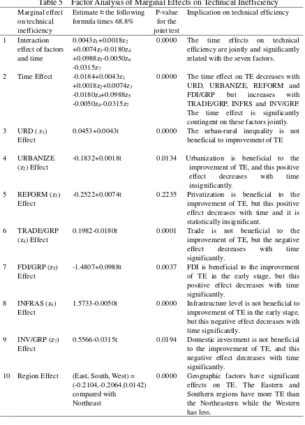
Table 5 Factor Analysis of Marginal Effects on Technical Inefficiency Marginal effect

on technical inefficiency

Estimate ≈ the following formula times 68.8%

P-value for the joint test

Implication on technical efficiency

1 Interaction effect of factors and time

0.0043z1+0.0018z2

+0.0074z3-0.0180z4

+0.0988z5-0.0050z6

-0.0315z7

0.0000 The time effects on technical efficiency are jointly and significantly related with the seven factors.

2 Time Effect -0.0184+0.0043z1

+0.0018z2+0.0074z3

-0.0180z4+0.0988z5

-0.0050z6-0.0315z7

0.0000 The time effect on TE decreases with URD, URBANIZE, REFORM and

FDI/GRP but increases with

TRADE/GRP, INFRS and INV/GRP. The time effect is significantly contingent on these factors jointly. 3 URD ( z1)

Effect

0.0453+0.0043t 0.0000 The urban-rural inequality is not

beneficial to improvement of TE

4 URBANIZE

(z2) Effect

-0.1832+0.0018t 0.0134 Urbanization is beneficial to the improvement of TE, and this positive

effect decreases with time

insignificantly. 5 REFORM (z3)

Effect

-0.2522+0.0074t 0.2235 Privatization is beneficial to the improvement of TE, but this positive effect decreases with time and it is statistically insignificant.

6 TRADE/GRP

(z4) Effect

0.1982-0.0180t 0.0001 Trade is not beneficial to the

improvement of TE, but the negative

effect decreases with time

significantly. 7 FDI/GRP (z5)

Effect

-1.4807+0.0988t 0.0037 FDI is beneficial to the improvement of TE in the early stage, but this positive effect decreases with time significantly.

8 INFRAS (z6)

Effect

1.5733-0.0050t 0.0000 Infrastructure level is not beneficial to improvement of TE in the early stage, but this negative effect decreases with time significantly.

9 INV/GRP (z7)

Effect

0.5566-0.0315t 0.0194 Domestic investment is not beneficial

to the improvement of TE, and this negative effect decreases with time significantly.

10 Region Effect (East, South, West) = (-0.2104,-0.2064,0.0142) compared with

Northeast

0.0000 Geographic factors have significant effects on TE. The Eastern and Southern regions have more TE than the Northeastern while the Western has less.

the estimated effect of urbanization on inefficiency is negative (-0.1832+0.0018t < 0).

This positive effect of urbanization on technical efficiency is statistically significant (the

probability value of the joint test is very small, shown in Row 4 of Table 5). Although

the effect decreases with time, it is both economically and statistically insignificant

since the coefficient estimate of “URBANIZE × t” is small and statistically

insignificant (see Table 4). The neoclassical analysis would argue that urbanization

enhances efficiency in two ways. On the one hand, people migrate to cities and obtain

better employment or wages, and hence higher savings, which in turn is converted into

productive investment capital and the technical efficiency can then be improved. On the

other hand, higher incomes also lead to changes in the composition of demand from

agricultural to manufactured goods. The demand of manufactured goods increases

technology and productivity growth.

As shown in Row 5 in Table 5, the REFORM factor shows a positive, albeit

insignificant, effect on technical efficiency. The REFORM factor is beneficial to TE

improvement (-0.2522+0.0074t < 0), but the effect on TE will finally become negative

with the development of privatization (when t>34, -0.2522+0.0074t >0). Although the

effect of privatization on efficiency is ambiguous in both theoretic and empirical

literatures (Okten and Arin, 2006), it is positive in our estimation. In China,

privatization has emancipated the productive forces which have been fettered by the

planned economy for a long time. Privatization can induce competition and enhance

productivity that eventually can contribute to efficiency improvement. However, even

though the effect is large, it is not statistically significant in our estimation since the

p-value of the test is 0.2235.

Trade and foreign investment can give rise to either positive or negative efficiency

(Loungani and Razin, 2001). Our estimates and tests in Rows 6 and 7 of Table 5 show

that in the early development stage TRADE/GRP has a negative and significant effect

on efficiency (0.1982-0.018t>0 when t<12), while FDI/GRP has a positive and

significant effect (-1.4807+0.0988t<0 when t<15). In the later development stage, the

effects will drive off in the reverse direction. One can see from Table 4 that the time

10 percent level, respectively. This may be due to two reasons. One is the problem of

endogeneity in the measurement of openness with the ratio of trade to GRP in the

growth literature. The other is that trade has been overemphasized in the economic

transition, while efficiency has artificially been ignored somewhat in China. For the

China’s economy to sustain a high-speed economic development, reform will have to

become a long-term policy, whereas international trade can be adjusted to suit for

growth and efficiency. Foreign direct investment can have an indirect effect on the

domestic economy via positive spillovers and competition (Blomstrom and Persson,

1983). Our finding implies that, even though FDI have an important and positive effect

on TE in the China’s economy, it should be further encouraged to neutralize the

downward trend of the effect.

The provision of infrastructure has a negative and significant effect on technical

efficiency (1.5733-0.005t>0), which implies that regional inequality in infrastructure

development in China has hindered improvement in technical efficiency. Although this

is inconsistent with the expectation about the positive effect of infrastructure on TE, it is

the regional bottleneck that constrains economic growth in China. To keep a balanced

growth among different regions, China should expand development in the

underdeveloped regions, especially the underprivileged regions in her western

provinces.

As regards to the domestic investment factor, our finding shows that it is only when

18

t that the effect of domestic investment on technical efficiency will be positive

(0.5566-0.0315t < 0). Thus, domestic investment is not beneficial to the improvement of

TE in the early stage of development (t<18). However, the time effect of the negative

marginal influence will significantly decrease with time (-0.0315<0). As we have found,

the effect of FDI on TE is contrary to the effect of domestic investment. The two kinds

of investment have direct and significant effects on TE for capital accumulation of the

local economy, but the direction of their effects is opposite to each other.

Finally, the result of Row 10 in Table 5 shows that geographic factors have a joint

significant effect on TE. The geographical location of a province in China can often

intermediate inputs and other resources. Thus, different geographic locations among the

provinces have different effects. When compared to the Northeastern region, the Eastern

and Southern / Western regions have a higher / lower technical efficiency. Consistent

with Figure 3, the ranking of technical efficiency for the four regions in China’s

economy is: East > South > Northeast > West.

6. Conclusion

This study uses a flexible stochastic production function to estimate technical

efficiency in China’s post-reform economy. A fully nonparametric time-variant

stochastic frontier model has been specified to allow for province effects and time

effects to enter the production function with other inputs in a nonparametric way. The

generalized kernel estimation is applied to smooth both the continuous input variables

and the categorical unordered provinces and the ordered time periods. The flexibility in

the production functional form and the manner of individual and time effects that

entered into the production model can minimize the loss in the measurement of

technical efficiency, lead to robust estimates of the frontier function and produce a

reliable measure of technical efficiency. Model specification tests and estimates show

that the fully nonparametric stochastic model is more suitable for our sample. The

average output elasticity of labor is larger than those of capital and human capital,

which are all positive.

The measure of TE based on nonparametric estimation shows that the average

technical efficiency in China has declined considerably in the mid-1980s, but has

increased since 1992. Technical efficiency tends to be higher than the national average

level in both Eastern and Southern regions. Although China has emphasized a lot on the

development of the Western region, its technical efficiency has remained low.

Unexpectedly, Beijing, being the capital of China, shows a lower technical efficiency

than most other provinces.

The estimation of the Tobit model of technical inefficiency shows that the time

contingent on the seven factors shown in Table 4. With the exception of privatization,

the marginal effects of all the other factors also have significant time effects. There

exists regional difference in technical efficiency. To maintain a sustainable, high-speed

development, China should continue to reform and adjust its international trade to suit

growth and efficiency improvement. Foreign direct investments have an important and

large positive effect on technical efficiency, but it should be further encouraged to

neutralize the downward trend of the effect. China should attach great importance to its

infrastructure policy and reappraise the infrastructure development policy to give a

positive effect on technical efficiency.

The empirical findings in this paper have improved the discussion on China’s

productivity analysis, echoed on such recent discussions as regional inequality, disparity

in growth inputs and human capital development in China’s post-reform economic

development (Wu, 2008; Li, 2009; Li and Liu, 2011; Chang, 2002; Fleisher and Zhao,

2010; Liu and Li, 2006; Chi, 2008; Li et al., 2009). Furthermore, the empirical findings

in this paper provide a reflection on the efficiency in financial issues, such as bank loans

and corporate bonds development, on economic policy decisions, such as the pace of

market liberalization and privatization of enterprises, and on infrastructural and civic

development, such as eradication of informal economic activities.

References

Balaguer-Coll, M. T., Prior, D. and Tortosa-Ausina, E. (2007). On the determinants of local government performance: a two-stage nonparametric approach. European Economic Review, 51(2), 425-451.

Barro, R. J., and Lee, J. W. (2001). International data for education attainment: Updates and Implications. Oxford Economics Papers, 3, 541-563.

Barro, R. J. and Sala-i-Martin, X. (1999). Economic Growth, Cambridge, Mass.: MIT Press.

Battese G. E. and Coelli, T. J. (1992). Frontier production functions, technical efficiency and panel data: With application to paddy farmers in India. Journal of Productivity Analysis, 3, 153-169.

Battese G. E. and Coelli, T. J. (1995). A model for technical inefficiency effects in a stochastic frontier production function for panel data. Empirical Economics, 20(2), 325-332.

Bauer, P. W. (1990). Decomposing TFP growth in the presence of cost inefficiency, non-constant return to scale, and technological progress. Journal of Productivity Analysis, 1, 287-299.

Benhabib, J. and Spiegel, M.M. (2005). Human capital and technology diffusion. In P. Aghion and S. Durlauf (eds.), Handbook of Economic Growth, North-Holland, Elsevier.

Blomstrom, M. and H. Persson, (1983). Foreign investment and spillover efficiency in an underdeveloped economy: Evidence from the Mexican manufacturing industries. World Development, 11, 493-501.

Borensztein, E. and Ostry, D. J. (1996). Accounting for China’s economic performance.

American Economic Review, 86, 224-228.

Bosworth, E., and Collins, S. M. (2008). Accounting for growth: comparing China and India. Journal of Economic Perspectives, 22 (1) Winter, 45-66.

Brummer, B., Clauben, T. and Lu, W. (2006). Policy reform and productivity change in Chinese agriculture: a distance function approach, Journal of Development Economics, 81, 61-79.

Chang, G. H. (2002). The cause and cure of China’s widening income disparity. China

Economic Review, 13, 335-340.

Chen, B.L. (2003). An inverted-U relationship between inequality and long-run growth. Economics Letters. 78, 205-212.

Chen , K., Huang Y., and Yang C. (2009). Analysis of regional productivity growth in China: A generalized metafrontier MPI approach. China Economic Review 20, pp. 777-792.

Chen, P., Yu, M., Chang, C., Hsu, S. (2008). Total factor productivity growth in China's agricultural sector. China Economic Review 19, pp.580-593.

Chi, Wei (2008). The role of human capital in China’s economic development:

review and new evidence. China Economic Review, 19, 421-436.

Chilingerian, J. A. (1995). Evaluating physician efficiency in hospitals: A multivariate

analysis of best practices. European Journal of Operational Research,80, 548-574.