Munich Personal RePEc Archive
Testing for a Deterministic Trend when
there is Evidence of Unit-Root
Gómez, Manuel and Ventosa-Santaulària, Daniel
Departamento de Economıa y Finanzas, Universidad de Guanajuato.
2010
Testing for a Deterministic Trend when there is
Evidence of Unit-Root
Manuel G´omez
∗Daniel Ventosa-Santaul`aria
†Revised version, 2010
Abstract
Whilst the existence of a unit root implies that current shocks have permanent ef-fects, in the long run, the simultaneous presence of a deterministic trend obliterates that consequence. As such, the long-run level of macroeconomic series depends upon the existence of a deterministic trend. This paper proposes a formal statistical procedure to distinguish between the null hypothesis of unit root and that of unit root with drift. Our procedure is asymptotically robust with regard to autocorre-lation and takes into account a potential single structural break. Empirical results show that most of the macroeconomic time series originally analysed by Nelson and Plosser (1982) are characterized by their containing both a deterministic and a stochastic trend.
Keywords:Unit Root, Deterministic Trend, Trend Regression,R2.
JEL Classification:C12, C13, C22.
1
Introduction
The influential paper by Nelson and Plosser (1982) (hereinafter NP) triggered a
con-siderable amount of research into the unit-root hypothesis on both the empirical and
the theoretical fronts. Since then, an impressive and increasingly complex array of
unit-root tests has been available in the literature, many of which were applied first to
the original NP dataset.
The significance of the debate lies in the effects of the stochastic shocks. Whenever
macroeconomic time series contain a unit root, random shocks have a permanent effect
∗Departamento de Econom´ıa y Finanzas, Universidad de Guanajuato.
†Corresponding Author: Departamento de Econom´ıa y Finanzas, Universidad de Guanajuato. Address:
on the series. However, in the long run, the effects of these shocks will be reduced if
the series also contains a deterministic trend.
The existence of a deterministic trend is also important for the limit distribution of
the unit root tests, since the distribution changes depending on the specification of
the deterministic component. Moreover, even though the existence of a deterministic
trend is more important for the long-run level of the series, there is a bias towards the
accurate analysis of the existence of a unit root, i.e. while most unit-root test procedures
include a deterministic trend regressor in their analysis, many of these do not formally
assess the performance of such estimate when there is evidence of unit root. Indeed,
Ventosa-Santaul`aria and G´omez (2007) proved that it is incorrect to carry out standard
hypothesis testing on the deterministic trend parameter estimated with Dickey-Fuller
(DF)-type tests when there is a unit root since the limiting distribution of its t-statistic
is neither asymptotically normal with unit variance nor nuisance-parameter-free when
the innovations are not i.i.d.
This implies that anyone interested in estimating the deterministic rate of growth of a
macroeconomic variable may find it difficult to perform such a task; although
seem-ingly straightforward, it becomes nontrivial when the series contains a unit root. In this
case, there is neither a reliable nor a simple tool available with which to carry out such
estimation.
This paper proposes a formal statistical procedure to distinguish between the null
hypothesis of unit root without drift and that of unit root with drift, with and
with-out a structural break [Note that the model under the alternative hypothesis of our
test corresponds to Perron’s Model B under the null hypothesis; see Perron (1989, p.
1364)]. Our work is in line with those that developed unit-root tests which also
con-sider a drift and a structural break under the null hypothesis; see, for example, Perron
(1989), Perron (1997), Carrion–i–Silvestre and Sans´o (2006), Kim and Perron (2009),
Carrion-i Silvestre, Kim, and Perron (2009), among others.1Nevertheless, these do not
focus on the estimation and hypothesis testing on the drift and the potential structural
break associated with it, but rather on the parameter associated with the autoregressive
term. Therefore, we believe that our procedure complements these unit-root tests
be-cause it formally concentrates on examining the presence of a deterministic trend and
a single structural break once there is evidence of a stochastic trend.2
In the empirical section, we enter the debate concerning the statistical properties of
the macroeconomic series of NP. When characterizing the series, we utilize a longer
span—updated to 1988—in order to benefit from the asymptotic properties of our
pro-cedure. In addition, we contrast our results with those of Perron (1997) and Carrion–i–Silvestre and Sans´o
(2006), who proposed unit-root tests that allow for a drift and a break under the null
hypothesis.
The article is organized as follows: in Section 2, we present a concise summary of the
best-known papers that analyse NP’s series. In Section 3, we derive the asymptotic
distribution of the new test under the null hypothesis, as well as under the relevant
alternative hypothesis, and tabulate the critical values for different levels. Section 4
presents a Monte Carlo exercise to evaluate the performance of this test in finite
sam-ples. Section 5 presents the empirical results for the NP dataset, whilst conclusions are
drawn in Section 6.
2
Literature Review
In this section, we briefly review the main findings of well-known papers that analyze
the unit-root hypothesis for the historical time series of NP.
In their seminal study, NP analyzed 14 US macroeconomic time series using Dickey and Fuller
(1979) unit-root test and failed to reject the null hypothesis of nonstationarity in all
only under the alternative hypothesis.
2All the unit-root tests so far mentioned consider a drift under the null hypothesis, consequently, if it
but one of the series, i.e. unemployment. Kwiatkowski, Phillips, Schmidt, and Shin
(1992) complemented existing unit-root tests by proposing a new procedure with trend
stationarity as the null hypothesis. They argued that the typical way in which this issue
is tested—unit root as the null hypothesis—causes the null hypothesis to be accepted
unless there is remarkable evidence against it; they could not actually reject the null
hypothesis of trend stationarity for unemployment, real per capita GNP, employment,
GNP deflator, wages and money stock. Perron (1989) extended the standard DF
proce-dure by adding dummy variables to allow for the presence of a one-time change in the
level or in the slope of the trend function under the alternative hypothesis or both. The
results showed that when the Great Depression and the first oil crisis in 1973 are treated
as points of structural change in the economy, it is possible to reject the null hypothesis
of unit root in favor of broken-trend stationary process—he could not reject the null
hypothesis in only 3 of the 14 series: CPI, velocity and bond yield. The assumption
that the location of the break is known a priori was criticized by several authors,
par-ticularly Christiano (1992), who argued that the choice of the break date is, in most
cases, correlated with the data. As a result, formal statistical test procedures capable
of determining breakpoints endogenously were proposed to test the unit-root
hypoth-esis. Zivot and Andrews (1992) proposed a Perron—type sequential test-applying his
methodology for each possible break date in the sample—applying his methodology
for each possible break date in the sample—that maximizes the evidence against the
null hypothesis of nonstationarity. They found less support in favor of broken-trend
stationarity than had Perron, rejecting the null hypothesis in only 7 of the original 14
series. Perron (1997) reconsidered his 1989 work by allowing endogenous breakpoint
determination. Most of the results in Perron (1989) were confirmed, although mixed
3
Identification of a deterministic trend in the presence
of a stochastic trend
Ventosa-Santaul`aria and G´omez (2007) proved that the DF-type test procedure may
fail to correctly identify the presence of a deterministic trend if the series also contains
a stochastic one.3 We propose an alternative procedure that can be used once there is
evidence in favor of unit root. Particularly, we are interested in distinguishing between:
• Driftless Unit Root:
H0: yt=Y0+ ξyt
|{z}
b
(1)
• Unit Root with drift:
Ha : yt=Y0+ µyt
|{z}
a
+ ξyt
|{z}
b
(2)
whereξyt =Pti=1uyi;uyirepresents the innovations and obeys the (general-level)
conditions stated in Phillips (1986, p. 313) and the underbraced components are
inter-preted as (a) Deterministic Trend, and (b) Stochastic Trend.
To distinguish betweenH0andHa, we will use the following auxiliary regression:
yt = γ+τ t+vt (3)
3.1
The case without structural breaks
Ifytis a unit root with drift process, then:
3The inference drawn from the t-ratio associated with the deterministic trend is misleading because it
Proposition 1 Letytbe generated by equation (1), and be used to estimate regression
(3). Hence, the associatedR2:
1. R2→d 1− Ω
R
ω2
−(R
ω)2 forµy= 0
2. R2= 1−O
p T−1
p
→1 forµy6= 0
whereΩ = R ω2 −4 Rω2 + 12R ωR rω−12 Rrω2. TheO
p T−1
term is
12−Ωσ2
lr µ2
y andσ
2
lris the long-run variance ofuyt.
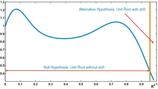
Proposition 1 implies that under H0, R2 converges to a degenerate and non-standard distribution and is always less than one, whereas under the relevant alternative
hypothesis,R2converges in probability to one. We computed the asymptotic
distribu-tion and estimated its shape non-parametrically (see Figure 1). The critical values are
also computed by simulating the asymptotic distribution. Actually, we simulated such
expression100,000times and obtained the relevant quantiles of the distribution (see
Table 1):
0 0.1 0.2 0.3 0.4 0.5 0.6 0.7 0.8 0.9 1
0.4 0.5 0.6 0.7 0.8 0.9 1 1.1 1.2 1.3
R2
Null Hypothesis: Unit Root without drift
Alternative Hypothesis: Unit Root with drift
[image:7.595.169.444.452.607.2]Level(α) 10% 5% 2.5% 1%
Critical Values atαlevel: 0.84 0.89 0.92 0.94
Table 1: Asymptotic critical values for theR2test
3.2
The case with structural breaks
All the asymptotics presented so far are made under the assumption that there are no
breaks in the series. Nevertheless, the vast literature concerning this issue favors the
hypothesis that structural breaks do occur occasionally in most economic series.
There-fore, our previous approach is generalized to allow a one-time change in the
determin-istic rate of growth, that is, our proposal accounts for one structural break that affects
only the slope of the time trend [Perron’s Model B under the null hypothesis (Perron,
1989, p. 1364)].
In doing so, we first show that the test, as originally proposed, no longer works
cor-rectly.4 Secondly, we modify the test regression to enable it to control for a possible break. Thirdly, we propose an algorithm that correctly identifies the break and thus
recovers the power of the test.
Assume now that the Data Generating Process (DGP) ofytis given by equation (4):
yt = µy+θyDUyt+yt−1+uyt (4)
= Y0+µyt+θyDTyt+ξyt
whereDUyt is a step dummy, that is,DUyt = 1(t > Tby), where1(·)is the
indi-cator function,Tby is the unknown date of the break iny,λ = Tby/T, andDTyt =
Pt
j=1DUyj is the deterministic trend structural break.
Running the test regression (3) on DGP (4) leads to erroneous inference. The R2
4Without any loss of generality we will assume thatythas a single break. The asymptotics for multiple
statistic behaves differently under the alternative hypothesis than has been previously
stated. In fact,R2does not converge to one under the alternative hypothesis, so the
two hypotheses become indistinguishable. There is a total loss of power. This result is
summarized in Proposition 2:
Proposition 2 Letytbe generated by equation (4), and be used to estimate regression
(3). Hence, the associatedR2:
R2→d 1−Op(1)<1
We may override this problem by running the test regression (5) on DGP (4) with a
correct specification of the break location:
yt = γ+τ t+πDTyt+vt (5)
The results stated in the previous section are once again valid, that is,R2 converges
to one in probability under the alternative hypothesis, as stated in Proposition 3. Note
that under the null hypothesis it is assumed that there is neither a drift nor a structural
break:
Proposition 3 Letytbe generated by equation (4), and be used to estimate regression
(5). Hence, the associatedR2:
1. R2→d 1−O
p(1) forµy=θy= 0
2. R2= 1−O
p T−1
p
→1 forµy6= 0andθy 6= 0
3. πˆ→p θy forµy6= 0andθy 6= 0
4. tπˆ=Op(T) forµy6= 0andθy 6= 0
As proved in the appendix, the asymptotic expressions under the null and the alternative
the limiting distribution under the null hypothesis depends upon the location of the
break.
Nevertheless, if we run a test regression (5) on DGP (4) with an incorrect specification
of the break location, as in equation (6), the test will fail again. LetTI
by 6=Tby, i.e.,T I by
denote an incorrect break date.
yt = γ+θt+τ DTytI +vt (6)
The test statistic,R2, does not converge to one under the alternative hypothesis. This
is stated in Proposition 4.
Proposition 4 Letytbe generated by equation (4), and be used to estimate regression
(6). Hence, the associatedR2:
R2 d
→1−Op(1)<1
Finally, if we include a break in the test regression and apply it to a series generated by
a DGP that does not have one, such test still works. Asymptotically, it does not matter
if a non-existent break is included:
Proposition 5 Letytbe generated by equation (1), and be used to estimate regression
(6). Hence, the associatedR2:
1. R2→d 1−O
p(1)<1 forµy =θy = 0
2. R2→p 1 forµ
y 6= 0andθy= 0
3. πˆ=Op
T−12
forµy =θy = 0
4. T−12t ˆ
π d
→Ψ forµy =θy = 0
whereΨis an unknown-nuisance-parameter-free distribution.
Given that our test statistic,R2, is asymptotically maximized when the break date is
it is possible to design a “break-finder” algorithm by running equation (6) sequentially
and allowing the break location to change along the sample. Eventually, if there is
indeed a break,R2will be maximized wheneverTI
by falls in the correct location and
will thus be equal toTby. More precisely, the break date is obtained by maximizing
(minimizing) theR2(sum of squared residuals, SSR):
ˆ
Tby =arg maxTby∈[εT ,(1−ε)T]R
2( ˆT
by)
whereTˆby is the estimated break date andε= 0.05is the trimming parameter.
It is important to note that, under the alternative hypothesis, we have not yet established
that our estimation method provides a consistent estimate of the break point.
Neverthe-less, we can make use of Perron and Zhu (2005) (PZ, hereinafter) results to assert that
this requirement is met since our estimation procedure matches one of their cases [our
DGP under the alternative hypothesis corresponds to PZ’s model I.a; refer to equation
(1) and assumption 2, pp. 69-70].5 PZ’s findings allow us to ensure that, under the
alternative hypothesis, our test consistently estimates the break date.6
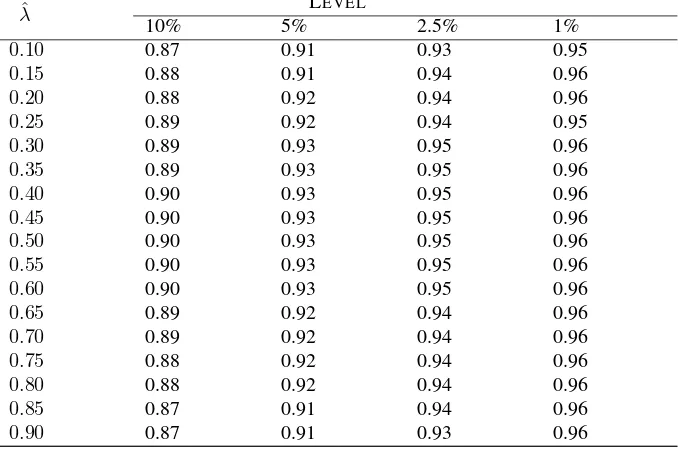
Under the null hypothesis there is no break but the auxiliary regression includes one
(located atTI
by). The asymptotic distribution under the null hypothesis is a function
of the—known—location of the break relative to the total sample (ˆλ= ˆTby/T). New
critical values that allow us to carry out hypothesis testing for given values ofλˆ are
thus tabulated in Table 2. These were computed for different break locations, ˆλ =
0.10,0.15,0.20,0.25, . . . ,0.85,0.90.
We also computed the distribution of√tπˆ
T. It contains no unknown nuisance parameters,
5PZ prove that a break fraction estimated by minimizing the SSR converges in probability—at a rate of
Op(T1/2)—to the true break fraction, whenever there is such a break [see Theorem 3 (1), p. 75]. Moreover,
they prove that the estimate associated to the trend break converges—at a rate ofOp(T1/2
)—to the true parameter if and only if, the break fraction is correct, which it is, given PZ’s previous result (refer to theorem 6 1(a), pp. 79). This implies that the break date estimate’s rate of convergence is fast enough to be considered as known
6Kim and Perron (2009) and Carrion-i Silvestre, Kim, and Perron (2009) also minimized the SSR; in
ˆ
λ LEVEL
10% 5% 2.5% 1%
0.10 0.87 0.91 0.93 0.95
0.15 0.88 0.91 0.94 0.96
0.20 0.88 0.92 0.94 0.96
0.25 0.89 0.92 0.94 0.95
0.30 0.89 0.93 0.95 0.96
0.35 0.89 0.93 0.95 0.96
0.40 0.90 0.93 0.95 0.96
0.45 0.90 0.93 0.95 0.96
0.50 0.90 0.93 0.95 0.96
0.55 0.90 0.93 0.95 0.96
0.60 0.90 0.93 0.95 0.96
0.65 0.89 0.92 0.94 0.96
0.70 0.89 0.92 0.94 0.96
0.75 0.88 0.92 0.94 0.96
0.80 0.88 0.92 0.94 0.96
0.85 0.87 0.91 0.94 0.96
[image:12.595.137.476.179.404.2]0.90 0.87 0.91 0.93 0.96
Table 2: Break location and asymptotic critical values for theR2test.
Note: the critical values are obtained from the simulation of the asymptotic distribution of the test statistic under the null hypothesis. Number of replications:20,000; the simulation of the Brownian motions is made exactly as in Perron (1989, p. 1375). Matlab code available upon request to the authors.
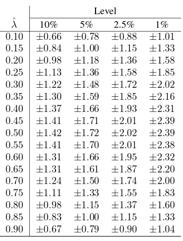
such asσ2
lr. Nevertheless, there is a known nuisance parameter—the estimated break
location (λˆ)—that alters this distribution. Therefore, we obtained critical values for
different break locations with which to test the null hypothesis:πˆ = 0;7 these critical values8appear in Table 3.
An example of the distribution of√tπˆ
T under the null hypothesis of non-significance is
shown in Figure 2. The specified break location isλˆ= 0.45.
7Thet-ratio associated with this parameter must be normalized byT12 in order to attain the asymptotic distribution underH0. Under the alternative hypothesis, thet-ratio diverges at rateT, so the square-root nor-malization factor does not impede its divergence; in fact, under the alternative hypothesis,√tˆπ
T =Op
T12
.
8The test is double-tailed; notice that the—non-standard—distribution appears to be symmetric. Note
also that the break date can be treated as known (under the alternative hypothesis) because of the same arguments stated for theR2
Level
ˆ
λ 10% 5% 2.5% 1%
[image:13.595.200.381.169.408.2]0.10 ±0.66 ±0.78 ±0.88 ±1.01 0.15 ±0.84 ±1.00 ±1.15 ±1.33 0.20 ±0.98 ±1.18 ±1.36 ±1.58 0.25 ±1.13 ±1.36 ±1.58 ±1.85 0.30 ±1.22 ±1.48 ±1.72 ±2.02 0.35 ±1.30 ±1.59 ±1.85 ±2.16 0.40 ±1.37 ±1.66 ±1.93 ±2.31 0.45 ±1.41 ±1.71 ±2.01 ±2.39 0.50 ±1.42 ±1.72 ±2.02 ±2.39 0.55 ±1.41 ±1.70 ±2.01 ±2.38 0.60 ±1.31 ±1.66 ±1.95 ±2.32 0.65 ±1.31 ±1.61 ±1.87 ±2.20 0.70 ±1.24 ±1.50 ±1.74 ±2.00 0.75 ±1.11 ±1.33 ±1.55 ±1.83 0.80 ±0.98 ±1.15 ±1.37 ±1.60 0.85 ±0.83 ±1.00 ±1.15 ±1.33 0.90 ±0.67 ±0.79 ±0.90 ±1.04
Table 3: Asymptotic critical values for√tπˆ
T.
Note: the critical values are obtained from the simulation of the asymptotic distribution of the test statistic under the null hypothesis [ˆπ= 0]. Number of replications:20,000; the simulation of the Brownian motions is made exactly as in Perron (1989, p. 1375). Matlab code available upon request to the authors.
−60 −4 −2 0 2 4 6
0.05 0.1 0.15 0.2 0.25 0.3 0.35 0.4 0.45 0.5
Sample distribution
Asymptotic Distribution
Figure 2: Asymptotic distribution of √tπˆ
[image:13.595.158.413.505.635.2]4
Finite-sample properties of the test
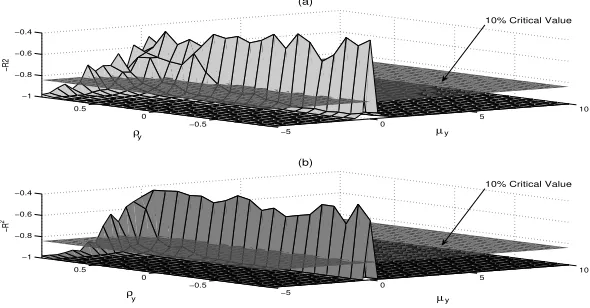
We present a Monte Carlo study to analyze the finite-sample effectiveness of the test. In
each case, the number of replications is1,000. Firstly, we evaluate the test performance
when no structural breaks are present in the data and the algorithm does not search
for breaks. Figure 3 shows the effect of autocorrelation9 on the behavior of the test
statistic for different values of the drift. This figure shows that autocorrelation has
only a marginal effect (for a10% level); the power of the test decreases slightly as
ρapproaches one. As the sample size increases, from T = 75 toT = 500, the
area with low power shrinks, although the gain in power seems to be relatively small.
Furthermore, there is a logical loss of power around the zero-valued drift, where the
null hypothesis is actually true.
−5
0
5 10 −0.5
0 0.5 −1 −0.8 −0.6 −0.4
µ
(a)
ρ
−R
2
−5 0
5 10 −0.5
0 0.5 −1 −0.8 −0.6 −0.4
µ
(b)
ρ
−R
2
10% Critical Value
10% Critical Value
y y
[image:14.595.157.452.416.570.2]y y
Figure 3:R2test-statistic in the presence of autocorrelation and for different values of the drift; (a)T = 75obs. and (b)T = 500obs.
More accurate Monte Carlo exercises are shown in Tables 4 and 5, in which the
rejec-tion rates of the null hypothesis for some selected parameter values, sample sizes and
statistical significance levels, are shown, these being:ρ= 0.0, 0.25, 0.5, 0.7 and 0.9; T
= 100, 150, 250, 500, 1,000; andα= 1%, and 5%, respectively.
Results show that the test is proficient for samples as small as one hundred
obser-vations. Where the DGP is a unit root without drift [Panels (a) of Tables 4 and 5],
rejection rates are as low as the significance levels for low values of the autocorrelation
coefficient (less than 0.5). In these cases, autocorrelation distortions may be assumed
to be unimportant. For values of the autocorrelation coefficient above 0.70, level
dis-tortions are important for sample sizes below 250. Where the DGP is a unit root with
drift [Panels (b)], the power of the test decreases when the drift approaches to zero and
autocorrelation is above 0.50. Although our test is asymptotically immune to
autocor-relation, the Monte Carlo experiments show that such immunity is not perfect in finite
samples, yet does work well for low levels of autocorrelation.
Secondly, we compare our test with that of Dickey and Fuller (1981) (hereinafter DF81).
DF81 specified a procedure to test the joint null hypothesis of unit root and the
non-significance of the deterministic regressors, in particular, the drift.
A comparison between DF81 and our test is not straightforward, since theR2test
pre-supposes that there is already evidence of unit root and focuses on testing the
signifi-cance of the deterministic components. However, our test may serve as a complement
when DF81 rejects the null hypothesis, as in those cases illustrated by Panels (b) of
Tables 6 and 7. When the underlying process is a unit root with drift, DF81
systemati-cally rejects the null hypothesis because it is half false [see Panels (b) of Tables 6 and
7].
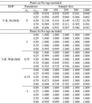
Furthermore, the Monte Carlo experiment reveals that the level distortions caused by
the presence of autocorrelation are more severe in the DF81 test [see Panel (a) of Table
6] than in theR2test [see Panels (a) of Tables 4 and 5]. Of course, Dickey-Fuller’s
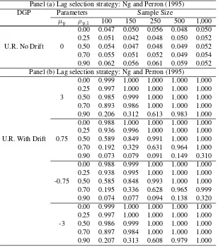
auxiliary regression can be adapted to control for autocorrelation; however, there is the
issue of selecting the number of lags to consider. We therefore applied Ng and Perron
Panel (a)
DGP Parameters Sample Size
µy ρy,1 100 150 250 500 1,000
0.00 0.011 0.009 0.010 0.010 0.010 0.25 0.013 0.011 0.011 0.011 0.010 U.R. No Drift 0 0.50 0.015 0.015 0.013 0.011 0.010 0.70 0.029 0.020 0.014 0.013 0.013 0.90 0.082 0.054 0.035 0.019 0.016
Panel (b)
U.R. With Drift
[image:16.595.134.446.171.523.2]0.00 1.000 1.000 1.000 1.000 1.000 0.25 1.000 1.000 1.000 1.000 1.000 3 0.50 1.000 1.000 1.000 1.000 1.000 0.70 0.999 1.000 1.000 1.000 1.000 0.90 0.707 0.776 0.891 0.984 0.999 0.00 0.993 0.999 1.000 1.000 1.000 0.25 0.928 0.984 0.999 1.000 1.000 0.75 0.50 0.660 0.823 0.948 0.998 1.000 0.70 0.315 0.415 0.606 0.869 0.986 0.90 0.139 0.128 0.123 0.170 0.280 0.00 0.993 0.999 1.000 1.000 1.000 0.25 0.932 0.983 0.999 1.000 1.000 -0.75 0.50 0.659 0.815 0.953 0.998 1.000 0.70 0.320 0.425 0.612 0.869 0.988 0.90 0.139 0.122 0.120 0.163 0.290 0.00 1.000 1.000 1.000 1.000 1.000 0.25 1.000 1.000 1.000 1.000 1.000 -3 0.50 1.000 1.000 1.000 1.000 1.000 0.70 0.999 1.000 1.000 1.000 1.000 0.90 0.697 0.771 0.889 0.983 0.999
Table 4: Rejection rates of theR2test. The case with no break (level:α= 0.01)
decreases the level distortions, however, it reduces the power of the test for high values
ofρ(above 0.50) and for low absolute values of the drift.10
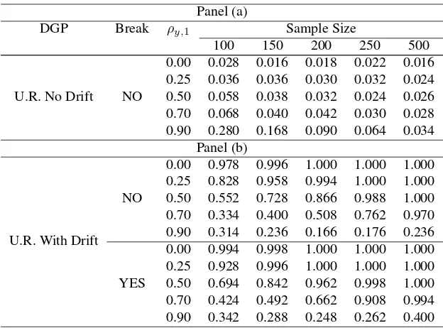
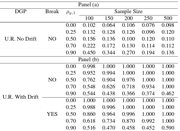
Thirdly, we assess the performance of the test when it searches for a single break in
the series. Tables 8 and 9 show the rejection rates of the null hypothesis when two
different DGPs are analyzed at the1%and5%levels. Panel (a) of each table—when
the DGP is unit root without drift—demonstrates that the test performs satisfactorily,
Panel (a)
DGP Parameters Sample Size
µy ρy,1 100 150 250 500 1,000
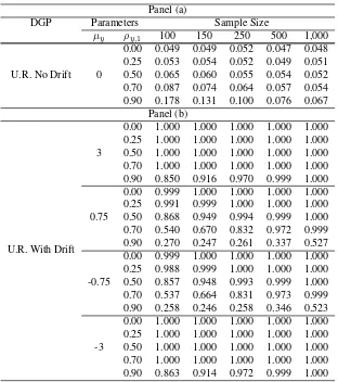
0.00 0.049 0.049 0.052 0.047 0.048 0.25 0.053 0.054 0.052 0.049 0.051 U.R. No Drift 0 0.50 0.065 0.060 0.055 0.054 0.052 0.70 0.087 0.074 0.064 0.057 0.054 0.90 0.178 0.131 0.100 0.076 0.067
Panel (b)
U.R. With Drift
[image:17.595.135.447.171.523.2]0.00 1.000 1.000 1.000 1.000 1.000 0.25 1.000 1.000 1.000 1.000 1.000 3 0.50 1.000 1.000 1.000 1.000 1.000 0.70 1.000 1.000 1.000 1.000 1.000 0.90 0.850 0.916 0.970 0.999 1.000 0.00 0.999 1.000 1.000 1.000 1.000 0.25 0.991 0.999 1.000 1.000 1.000 0.75 0.50 0.868 0.949 0.994 0.999 1.000 0.70 0.540 0.670 0.832 0.972 0.999 0.90 0.270 0.247 0.261 0.337 0.527 0.00 0.999 1.000 1.000 1.000 1.000 0.25 0.988 0.999 1.000 1.000 1.000 -0.75 0.50 0.857 0.948 0.993 0.999 1.000 0.70 0.537 0.664 0.831 0.973 0.999 0.90 0.258 0.246 0.258 0.346 0.523 0.00 1.000 1.000 1.000 1.000 1.000 0.25 1.000 1.000 1.000 1.000 1.000 -3 0.50 1.000 1.000 1.000 1.000 1.000 0.70 1.000 1.000 1.000 1.000 1.000 0.90 0.863 0.914 0.972 0.999 1.000
Table 5: Rejection rates of theR2test. The case with no break (level:α= 0.05)
particularly when the inference is drawn based on a 1% level; rejection rates under the
null hypothesis are fairly low even for small samples when autocorrelation is low. Panel
(b) of each table—when the DGP is unit root with drift—shows high rejection rates of
the null hypothesis in both cases, i.e. when the DGP has no break, and when it does.
Nevertheless, it is noticeable that positive autocorrelation may have a considerable
negative effect on the power of the test in relatively small samples, i.e., those with
Panel (a) No lags included
DGP Parameters Sample Size
µy ρy,1 100 150 250 500 1,000
0.00 0.034 0.038 0.045 0.041 0.048 0.25 0.058 0.055 0.060 0.066 0.062 U.R. No Drift 0 0.50 0.138 0.141 0.149 0.152 0.158 0.70 0.289 0.292 0.311 0.302 0.301 0.90 0.606 0.591 0.587 0.586 0.583 Panel (b) No lags included
[image:18.595.136.446.170.522.2]0.00 1.000 1.000 1.000 1.000 1.000 0.25 1.000 1.000 1.000 1.000 1.000 3 0.50 1.000 1.000 1.000 1.000 1.000 0.70 1.000 1.000 1.000 1.000 1.000 0.90 0.995 0.999 1.000 1.000 1.000 0.00 1.000 1.000 1.000 1.000 1.000 0.25 0.999 1.000 1.000 1.000 1.000 U.R. With Drift 0.75 0.50 0.980 0.998 1.000 1.000 1.000 0.70 0.880 0.949 0.992 1.000 1.000 0.90 0.703 0.725 0.796 0.884 0.965 0.00 1.000 1.000 1.000 1.000 1.000 0.25 0.999 1.000 1.000 1.000 1.000 -0.75 0.50 0.981 0.998 1.000 1.000 1.000 0.70 0.873 0.949 0.993 1.000 1.000 0.90 0.698 0.738 0.782 0.885 0.969 0.00 1.000 1.000 1.000 1.000 1.000 -3 0.25 1.000 1.000 1.000 1.000 1.000 0.50 1.000 1.000 1.000 1.000 1.000 0.70 1.000 1.000 1.000 1.000 1.000 0.90 0.995 0.999 1.000 1.000 1.000
Table 6: Rejection rates of Dickey-Fuller’s (1981) joint test: the case with no break. Lags not included, level:α= 0.05
5
Empirical results for Nelson and Plosser series
The purpose of this section is twofold. Firstly, we use our new test to review the
statistical properties of the NP series. We apply the popular Zivot and Andrews (1992)
test, since our test is properly used only after a unit-root test has been employed. If the
former fails to reject the null hypothesis of nonstationarity, then our test can be used.11
11Although Zivot and Andrews’s (1992) test does not allow for a structural break under the null hypothesis
of unit root, Vogelsang and Perron (1998) argue on pp. 1092-1093 that: “asymptotic results—[assuming a
distribu-Panel (a) Lag selection strategy: Ng and Perron (1995)
DGP Parameters Sample Size
µy ρy,1 100 150 250 500 1,000
0.00 0.047 0.050 0.056 0.048 0.050 0.25 0.051 0.042 0.048 0.050 0.052 U.R. No Drift 0 0.50 0.054 0.047 0.048 0.049 0.052 0.70 0.055 0.051 0.052 0.049 0.054 0.90 0.062 0.056 0.061 0.059 0.052 Panel (b) Lag selection strategy: Ng and Perron (1995)
[image:19.595.139.447.174.524.2]0.00 0.999 1.000 1.000 1.000 1.000 0.25 0.997 1.000 1.000 1.000 1.000 3 0.50 0.985 0.999 1.000 1.000 1.000 0.70 0.893 0.986 1.000 1.000 1.000 0.90 0.206 0.312 0.613 0.983 1.000 0.00 0.988 1.000 1.000 1.000 1.000 0.25 0.936 0.996 1.000 1.000 1.000 U.R. With Drift 0.75 0.50 0.589 0.849 0.991 1.000 1.000 0.70 0.192 0.329 0.631 0.964 1.000 0.90 0.073 0.079 0.091 0.149 0.310 0.00 0.988 0.999 1.000 1.000 1.000 0.25 0.938 0.995 1.000 1.000 1.000 -0.75 0.50 0.585 0.848 0.993 1.000 1.000 0.70 0.195 0.336 0.628 0.965 0.999 0.90 0.074 0.077 0.094 0.138 0.320 0.00 0.999 1.000 1.000 1.000 1.000 0.25 0.997 1.000 1.000 1.000 1.000 -3 0.50 0.986 0.999 1.000 1.000 1.000 0.70 0.897 0.984 1.000 1.000 1.000 0.90 0.207 0.313 0.608 0.979 1.000
Table 7: Rejection rates of Dickey-Fuller’s (1981) joint test: the case with no break. Lag selection strategy: Ng and Perron (2005), level:α= 0.05
Secondly, we contrast our results with those obtained by unit-root tests which include
a break under the null hypothesis: Perron (1997) and Carrion–i–Silvestre and Sans´o
(2006) [hereinafterP97andCS06, respectively]. P97andCS06proposed models
that differ on whether or not there is a break under the null hypothesis and the type of
break. The specific models that they selected in their empirical applications inhibits the
Panel (a)
DGP Break ρy,1 Sample Size
100 150 200 250 500
U.R. No Drift NO
0.00 0.028 0.016 0.018 0.022 0.016 0.25 0.036 0.036 0.030 0.032 0.024 0.50 0.058 0.038 0.032 0.024 0.026 0.70 0.068 0.040 0.042 0.030 0.028 0.90 0.280 0.168 0.090 0.064 0.034
Panel (b)
U.R. With Drift NO
0.00 0.978 0.996 1.000 1.000 1.000 0.25 0.828 0.958 0.994 1.000 1.000 0.50 0.552 0.728 0.866 0.988 1.000 0.70 0.334 0.400 0.508 0.762 0.970 0.90 0.314 0.236 0.166 0.176 0.236
YES
[image:20.595.135.447.172.403.2]0.00 0.994 0.998 1.000 1.000 1.000 0.25 0.928 0.996 1.000 1.000 1.000 0.50 0.694 0.842 0.962 0.998 1.000 0.70 0.424 0.492 0.662 0.908 0.994 0.90 0.342 0.288 0.248 0.262 0.400
Table 8: Rejection rates of the R2 test. The case with breaka (Level: α = 0.01;
trimming:ε= 0.05)
aIn all cases, there is a grid search for a break;µy = 2.7,σy = 5, and, if the DGP contains a break:
θy= 1.05,λ= 0.5.
comparison with the results of our test.12Therefore, we compute their results choosing
those models that allow us to make the fairest comparison with our test.13 In particular,
we apply Perron´s model B14to all the series under analysis; this model is referred as
the “changing growth model”. Under the null hypothesis, it permits a change in the
trend function without any change in the level at the time of the break. We also apply
the model thatCS06denominatedΘ5,1(λ). This particular specification allows a slope
shift under the null hypothesis.
We employ the NP series updated to1988by Herman van Dijk that can be found in
the JBES 1994 dataset archives; we expect the longer span to make the results more
12We previoulsly warned that a comparison between our test and any root test is not straightforward, given
that our test assumes that there is evidence of unit root and tests the significance of the drift, whilstP97and
CS06test the unit root hypothesis.
13We used the test statistics,t∗
α(3)ofP97andΘ5,1(λ)ofCS06; both allow for a change in the time trend [Model B in Perron’s (1989) notation]. The Matlab code is available upon request.
Panel (a)
DGP Break ρy,1 Sample Size
100 150 200 250 500
U.R. No Drift NO
0.00 0.102 0.064 0.106 0.076 0.098 0.25 0.132 0.128 0.126 0.096 0.120 0.50 0.156 0.136 0.100 0.120 0.110 0.70 0.222 0.172 0.130 0.114 0.112 0.90 0.450 0.344 0.270 0.194 0.136
Panel (b)
U.R. With Drift NO
0.00 0.998 1.000 1.000 1.000 1.000 0.25 0.952 0.994 1.000 1.000 1.000 0.50 0.762 0.904 0.976 1.000 1.000 0.70 0.548 0.626 0.718 0.934 1.000 0.90 0.544 0.438 0.366 0.374 0.462
YES
[image:21.595.137.451.172.401.2]0.00 1.000 1.000 1.000 1.000 1.000 0.25 0.988 0.996 1.000 1.000 1.000 0.50 0.860 0.964 0.996 1.000 1.000 0.70 0.618 0.734 0.870 0.992 1.000 0.90 0.516 0.470 0.458 0.452 0.590
Table 9: Rejection rates of the R2 test. The case with breaka (Level: α = 0.05;
trimming:ε= 0.05)
aIn all cases, there is a grid search for a break;µy = 2.7,σy = 5, and, if the DGP contains a break:
θy= 1.05,λ= 0.5.
reliable. The data are annual and all the series are in natural logs except for that of
bond yield.
The results in Table 10 show that for all variables except real GNP, nominal GNP
and real per capita GNP, there is insufficient evidence to reject the null hypothesis
of unit root. Therefore, these three variables can be considered broken-trend stationary
series. The remaining variables in Table 10 are appropriate candidates for the procedure
developed in this paper, since there is evidence in favor of unit root. We are able to
reject the null hypothesis of driftless unit root for all the series except CPI, velocity,
bond yield and stock prices.
For the remainder—industrial production, employment, deflator, nominal wages, real
wages and money stock—there is evidence to affirm that these are governed by a
Series ZAa Break R2
Break P97 CS06 location location t∗
α(3) Θ5,1(λ)
Real GNP -5.542** 1934 — — 1930 1978***
Nominal GNP -5.734*** 1930 — — 1939 1928*** Real per capita GNP -5.860*** 1939 — — 1930 1937 Industrial Production -4.939 1919 0.988*** 1901 1897 1917*** Employment -4.748 1930 0.972*** 1906 1904 1943*** GNP deflator -3.813 1930 0.921** 1965*** 1953 1918***
CPI -2.284 1931 0.726 — 1953 1871***
Wages -4.889 1930 0.967*** 1940 1943 1920*** Real Wages -3.653 1972 0.978*** 1973** 1971 1973*** Money Stock -4.451 1929 0.986*** 1970 1970 1978***
Velocity -4.030 1930 0.927 — 1936 1928***
[image:22.595.147.463.172.320.2]Bond Yield -4.191 1954 0.857 — 1954 1931** Stock Prices -4.476 1954 0.873 — 1942* 1928***
Table 10: Extended NP data set
aZivot and Andrews’s (1992)t-statistic associated with autoregressive term, Model (C).
Trimming:ε= 0.05; Breaks allowed: level and trend; lags selected by the Akaike Information Criterion. The symbols *, **, and *** denote rejection of the null hypothesis at 10%, 5%, and 1% level, respectively.
structural breaks in the deterministic trend of real wages(1973)and deflator(1965).
Results in the Monte Carlo section show that the test loses some power in the
pres-ence of positive autocorrelation for sample sizes below200. Notwithstanding, the test
still has enough power to reject the null hypothesis in all but four cases. Furthermore,
the combined results ofP97andCS06tests for the series, industrial production,
em-ployment, GNP deflator, wages, real wages and money stock, can be interpreted and
reconciled as follows. For all these series, theP97test does not reject the null
hypoth-esis of unit root, whereas theCS06test does reject the null; theCS06test rejects the
null because one or more of the constraints related to the slope or the slope shift are not
met, and not necessarily because of the absence of a unit root. These results imply the
presence of a unit root and the absence of a drift/drift and shift, among others. Since
our test also rejects the null hypothesis, we can conclude that all these series contain
both, a deterministic and a stochastic trend. Moreover, besides the deterministic trend,
our test shows that the GNP deflator and real wages also have a structural break in the
deterministic rate of growth. The application of our test further refines the results of
those ofP97andCS06tests. For example, the modelΘ5,1(λ)of CS06tests under
there-fore, if the null hypothesis is rejected, it is not possible to tell which of the constraints
are not true. By using our test, it is possible to draw inference about the deterministic
components, specifically, the deterministic trend or the structural break associated with
it.
6
Concluding remarks
This work aims to complement unit-root literature by proposing a new and simple
methodology that provides a correct assessment of the deterministic trend when there
is evidence of unit root. Our procedure contributes by increasing the degree of
preci-sion in the inference drawn from unit-root tests that consider drift and break under the
null hypothesis. For these tests, it is impossible to evaluate whether both the drift and
the break are simultaneously present whenever the null of nonstationarity cannot be
re-jected, whereas our methodology provides a simple and reliable approach to executing
this task.
The importance of such an assessment relies on the fact that existing unit-root tests
fail to correctly estimate the existence of the deterministic trend under the null
hypoth-esis of unit root; therefore, the literature lacks a reliable tool with which to estimate
the deterministic rate of growth of a series when a stochastic trend exists. The
pro-cedure is simple and its implementation straightforward; furthermore, it facilitates the
interpretation of the dynamics of the macroeconomic and financial time series.
The new procedure is shown to be asymptotically robust with regard to autocorrelation,
and to have reasonable power for sample sizes of practical interest. We considered
the possibility of a single structural break in the deterministic trend and derived the
asymptotic distribution of both theR2statistic as well as thet-statistic associated with
the structural break parameter estimated under the null hypothesis of no break.
The empirical results show that most of the NP series extended up to 1988—with the
containing a deterministic trend. The results of Perron (1997) test using his “changing
growth” model are in line with ours since there is not enough evidence against the
unit-root hypothesis in all cases but one. For these variables, our test clarifies that there is a
deterministic trend besides the unit root.
References
CARRION–I–SILVESTRE, J.,ANDA. SANSO´ (2006): “Joint hypothesis specification for unit root tests with a structural break,”Econometrics Journal, 9(2), 196–224.
CARRION-ISILVESTRE, J., D. KIM,ANDP. PERRON(2009): “GLS-Based Unit Root
Tests with Multiple Structural Breaks Under Both the Null and the Alternative
Hy-potheses,”Econometric Theory, 25(06), 1754–1792.
CHRISTIANO, L. (1992): “Searching for a Break in GNP,”Journal of Business &
Economic Statistics, 10(3), 237–250.
DICKEY, D.,ANDW. FULLER(1979): “Distribution of the Estimators for
Autoregres-sive Time Series With a Unit Root,”Journal of the American Statistical Association,
74(366), 427–431.
(1981): “Likelihood Ratio Statistics for Autoregressive Time Series with a
Unit Root,”Econometrica, 49(4), 1057–1072.
HAMILTON, J. (1994):Time Series Analysis. Princeton University Press.
KIM, D., ANDP. PERRON(2009): “Unit root tests allowing for a break in the trend
function at an unknown time under both the null and alternative hypotheses,”Journal
of Econometrics, 148(1), 1–13.
KWIATKOWSKI, D., P. PHILLIPS, P. SCHMIDT, ANDY. SHIN(1992): “Testing the
null hypothesis of stationarity against the alternative of a unit root,” Journal of
NELSON, C., AND C. PLOSSER (1982): “Trends and Random Walks in
Macroeco-nomic Time Series,”Journal of Monetary Economics, 10, 139–162.
NG, S., AND P. PERRON (1995): “Unit root tests in ARMA models with data-dependent methods for the selection of the truncation lag,”Journal of the American
Statistical Association, pp. 268–281.
PERRON, P. (1989): “The Great Crash, the Oil Price Shock and the Unit Root
Hypoth-esis,”Econometrica, 57, 1361–1401.
(1997): “Further Evidence on breaking Trend Functions in Macroeconomic
Variables,”Journal of Econometrics, 80, 335–385.
PERRON, P.,ANDX. ZHU(2005): “Structural breaks with deterministic and stochastic
trends,”Journal of Econometrics, 129(1-2), 65–119.
PHILLIPS, P. (1986): “Understanding Spurious Regressions in Econometrics,”Journal
of Econometrics, 33(3), 311–40.
PHILLIPS, P.,ANDS. DURLAUF(1986): “Multiple Time Series Regression with
Inte-grated Processes,”The Review of Economic Studies, 53(4), 473–495.
VENTOSA-SANTAULARIA, D.,` ANDM. G ´OMEZ(2007): “Income Convergence: The Validity of the Dickey-Fuller Test Under the Simultaneous Presence of Stochastic
and Deterministic Trends,”Guanajuato School of Economics Working Paper Series,
EM200703.
VOGELSANG, T.,ANDP. PERRON(1998): “Additional tests for a unit root allowing for
a break in the trend function at an unknown time,”International Economic Review,
39(4).
ZIVOT, E., AND D. ANDREWS (1992): “Further Evidence on the Great Crash, the
Oil-Price Shock, and the Unit-Root Hypothesis,”Journal of Business & Economic
A
Appendix
Proof of Propositions 1-5.We present a guide on how to obtain the order in probability
of one combination of DGP and specification, namely DGP (1) and specification (4).
The expressions needed to compute the asymptotic value ofR2are:
X
yt = Y0T+µy
X
t+Xξy,t−1
| {z }
Op T 3 2 X
ytt = Y0
X
t+µy
X
t2+Xξy,t−1t
| {z }
Op
T52
X
y2t = Y02T+µ2y
X
t2+Xξy,t2 −1
| {z }
Op(T2)
+2Y0µy
X
t+...
2Y0
X
ξy,t−1+ 2µy
X
ξy,t−1t
X
t = 1
2 T
2+T
X
t2 = 1
6 2T
3+ 3T2+T
whereξy,t =Pti=1uy,i and all other summations range from1toT. The orders in
probability can be found in Phillips (1986), Phillips and Durlauf (1986) and Hamilton
(1994). These expressions were written inMathematica 4.1code; the software
com-putes the asymptotics of the classical OLS formula(X′X)−1X′Y as well as the
asymp-totic value of the variance estimator:σb2
u=T−1
PT
t=1bu2t where.
X′X =
T P t P
t Pt2
and, Y = P yt P
ytt
The code in this case15 is represented below. To understand it, a brief glossary is
required:
Character Represents
A Y0
K µy
B P
ξy,t−1
C P
ξ2
y,t−1
D P
ξy,t−1t
St P
t
St2 P
[image:27.595.260.353.297.381.2]t2
Table 11: glossary of the Mathematica Code
ClearAll;St=12∗(T2+T);St2= 1
6∗(2∗T3+ 3∗T2+T); ClearAllClearAll;;StSt== 2121∗∗((TT22++TT););St2St2==116∗(2∗T3+ 3∗T2+T);
6∗(2∗T3+ 3∗T2+T); Sy=A∗T+K∗St+B∗T1.5;
Sy=A∗T+K∗St+B∗T1.5; Sy=A∗T+K∗St+B∗T1.5;
Sy2=A2∗T+K2∗St2+C∗T2+ 2∗A∗K∗St+ 2∗A∗B∗T1.5 Sy2=A2∗T+K2∗St2+C∗T2+ 2∗A∗K∗St+ 2∗A∗B∗T1.5 Sy2=A2∗T+K2∗St2+C∗T2+ 2∗A∗K∗St+ 2∗A∗B∗T1.5
+2∗K∗D∗T2.5;
+2+2∗∗KK∗∗DD∗∗TT22..55;;
Syt=A∗St+K∗St2+D∗T2.5; SytSyt==AA∗∗StSt++KK∗∗St2St2++DD∗∗TT22..55;;
Mx= ( T St
St St2
);
Mx= ( T St
St St2
);
Mx= ( T St
St St2
);
iMx=Inverse[Mx];
iMxiMx==InverseInverse[[MxMx];];
R1=Extract[iMx,{1,1}];R2=Extract[iMx,{1,2}];
R1R1==ExtractExtract[[iMxiMx,,{{11,,11}}];];R2R2==ExtractExtract[[iMxiMx,,{{11,,22}}];];
R3=Extract[iMx,{2,1}];R4=Extract[iMx,{2,2}];
R3R3==ExtractExtract[[iMxiMx,,{{22,,11}}];];R4R4==ExtractExtract[[iMxiMx,,{{22,,22}}];];
R40=Factor[R4];
R40R40==FactorFactor[[R4R4];];
R4num=Numerator[R40];
R4numR4num==NumeratorNumerator[[R40R40];];
R4den=Denominator[R40];
R4denR4den==DenominatorDenominator[[R40R40];];
15As indicated previously, the proof was achieved with the aid ofMathematica 4.1software. The
K15=Exponent[R4num, T];
K15K15==ExponentExponent[[R4numR4num, T, T];];
K16=Exponent[R4den, T];
K16K16==ExponentExponent[[R4denR4den, T, T];];
R4num2=Limit[Expand[R4num/TK15], T → ∞];
R4num2=Limit[Expand[R4num/TK15], T → ∞];
R4num2=Limit[Expand[R4num/TK15], T → ∞];
R4den2=Limit[Expand[R4den/TK16], T → ∞];
R4den2=Limit[Expand[R4den/TK16], T → ∞];
R4den2=Limit[Expand[R4den/TK16], T → ∞];
R42=Factor[Expand[(R4num2/R4den2)∗ TTK15K16]]; R42=Factor[Expand[(R4num2/R4den2)∗ TK15
TK16]]; R42=Factor[Expand[(R4num2/R4den2)∗TTK15K16]];
P10=Factor[Expand[R1∗Sy+R2∗Syt]];
P10P10==FactorFactor[[ExpandExpand[[R1R1∗∗SySy++R2R2∗∗SytSyt]];]];
P20=Factor[Expand[R3∗Sy+R4∗Syt]];
P20P20==FactorFactor[[ExpandExpand[[R3R3∗∗SySy++R4R4∗∗SytSyt]];]];
P21num=Numerator[P20];
P21numP21num==NumeratorNumerator[[P20P20];];
K3=Exponent[P21num, T];
K3K3==ExponentExponent[[P21numP21num, T, T];];
Bnum=Limit[Expand[P21num/TK3], T → ∞];
Bnum=Limit[Expand[P21num/TK3], T → ∞];
Bnum=Limit[Expand[P21num/TK3], T → ∞];
P22den=Denominator[P20];
P22denP22den==DenominatorDenominator[[P20P20];];
K4=Exponent[P22den, T];
K4K4==ExponentExponent[[P22denP22den, T, T];];
Bden=Limit[Expand[P22den/TK4], T → ∞];
BdenBden==LimitLimit[[ExpandExpand[[P22denP22den/T/TK4K4]], T, T → ∞→ ∞];];
Bpar=Factor[Expand[(Bnum/Bden)∗ TK3
TK4]]; Bpar=Factor[Expand[(Bnum/Bden)∗TK3
TK4]]; Bpar=Factor[Expand[(Bnum/Bden)∗ TK3
TK4]];
P40=FactorExpandSy2+P102∗T+P202∗St2 P40P40==FactorFactorExpandExpandSy2Sy2++P10P1022∗∗TT++P20P2022∗∗St2St2
−2∗P10∗Sy−2∗P20∗Syt+ 2∗P10∗P20∗St]] ;
−2∗P10∗Sy−2∗P20∗Syt+ 2∗P10∗P20∗St]] ;
−2∗P10∗Sy−2∗P20∗Syt+ 2∗P10∗P20∗St]] ;
P41num=Numerator[P40];
P41numP41num==NumeratorNumerator[[P40P40];];
K7=Exponent[P41num, T];
K7K7==ExponentExponent[[P41numP41num, T, T];];
U2num=Factor[Limit[Expand[P41num/TK7], T → ∞]];
U2num=Factor[Limit[Expand[P41num/TK7], T → ∞]];
U2num=Factor[Limit[Expand[P41num/TK7], T → ∞]];
P42den=Denominator[P40];
P42denP42den==DenominatorDenominator[[P40P40];];
K8=Exponent[P42den, T];
K8K8==ExponentExponent[[P42denP42den, T, T];];
U2den=Factor[Limit[Expand[P42den/TK8], T → ∞]];
U2denU2den==FactorFactor[[LimitLimit[[ExpandExpand[[P42denP42den/T/TK8K8]], T, T → ∞→ ∞]];]];
Su2=FullSimplify[Factor[Expand[(U2num/U2den)∗TK7
TK8]]]; Su2=FullSimplify[Factor[Expand[(U2num/U2den)∗ TK7
TK8]]]; Su2=FullSimplify[Factor[Expand[(U2num/U2den)∗ TK7
P50=Factor[Expand[P40/(Sy2+T∗(SyT)2−2∗(Sy
T)∗Sy)]];
P50P50==FactorFactor[[ExpandExpand[[P40P40//((Sy2Sy2++TT∗∗((SySyTT))22−−22∗∗((SySyT)∗Sy)]];
T)∗Sy)]];
P51num=Numerator[P50];
P51numP51num==NumeratorNumerator[[P50P50];];
K1=Exponent[P51num, T];
K1K1==ExponentExponent[[P51numP51num, T, T];];
Rcnum=Factor[Limit[Expand[P51num/TK1], T → ∞]];
Rcnum=Factor[Limit[Expand[P51num/TK1], T → ∞]];
Rcnum=Factor[Limit[Expand[P51num/TK1], T → ∞]];
P52den=Denominator[P50];
P52denP52den==DenominatorDenominator[[P50P50];];
K2=Exponent[P52den, T];
K2K2==ExponentExponent[[P52denP52den, T, T];];
Rcden=Factor[Limit[Expand[P52den/TK2], T → ∞]];
Rcden=Factor[Limit[Expand[P52den/TK2], T → ∞]];
Rcden=Factor[Limit[Expand[P52den/TK2], T → ∞]];
Rc=FullSimplify[Factor[Expand[(Rcnum/Rcden)∗TK1
TK2]]] Rc=FullSimplify[Factor[Expand[(Rcnum/Rcden)∗ TK1
TK2]]] Rc=FullSimplify[Factor[Expand[(Rcnum/Rcden)∗ TK1