http://dx.doi.org/10.4236/ajor.2013.36050
Adaptive Strategies for Accelerating the Convergence of
Average Cost Markov Decision Processes Using a Moving
Average Digital Filter
Edilson F. Arruda1, Fabrício Ourique2
1Federal University of Rio de Janeiro, Alberto Luiz Coimbra Institute—Graduate School and Research in Engineering, Rio de Janeiro, Brazil
2Federal University of Santa Catarina (Campus Araranguá), Araranguá, Brazil Email: [email protected]
Received July 9, 2013; revised August 9, 2013; accepted August 16,2013
Copyright © 2013 Edilson F. Arruda, Fabrício Ourique. This is an open access article distributed under the Creative Commons At- tribution License, which permits unrestricted use, distribution, and reproduction in any medium, provided the original work is prop- erly cited.
ABSTRACT
This paper proposes a technique to accelerate the convergence of the value iteration algorithm applied to discrete aver- age cost Markov decision processes. An adaptive partial information value iteration algorithm is proposed that updates an increasingly accurate approximate version of the original problem with a view to saving computations at the early iterations, when one is typically far from the optimal solution. The proposed algorithm is compared to classical value iteration for a broad set of adaptive parameters and the results suggest that significant computational savings can be obtained, while also ensuring a robust performance with respect to the parameters.
Keywords: Average Cost; Markov Decision Processes; Value Iteration; Computational Effort; Gradient
1. Introduction
Discrete-time Markov decision processes aim at control- ling the dynamics of a stochastic system by mean of tak- ing suitable control actions at each possible configuration of the system. At each period, a control action is selected based on the current configuration (state) of the system, which triggers a probabilistic transition to another state in the next decision period and so on in an infinite time horizon. The objective is to find the best action to be taken at each possible configuration of the system with respect to some prescribed performance measure. From now on, each configuration of the system is referred to as a state of the system.
An elegant way to find the optimal control actions for each state is provided by the classical value or policy iteration algorithms [1-11]. The value iteration (VI) algo- rithm is arguably the most popular algorithm, in part be- cause of its simplicity and ease of implementation. In this paper, we introduce an adaptive way to improve the con- vergence of the VI algorithm with respect to conver- gence time, with a view at accelerating the convergence of the method. We refer to [12] for a study on variants of
the policy iteration algorithm.
We explore a way to accelerate the convergence of val- ue iteration algorithms for average cost MDPs. The ra- tionale is to apply the value iteration algorithm to a se- quence of approximate models, which are simpler than the original model and hence require less computation. These models are refined at each new iteration of the algorithm and converge to the exact model within a finite number of iterations, which enables one to retrieve the solution to the original problem at the end of the proce- dure. The rationale is based on a refinement scheme in- troduced in [13] for linearly convergent algorithms with convergence rates that are known a priori.
such rate is now known a priori and the parameter tuning turns out to be very difficult. Moreover, consistent per- formance gains over the classical VI algorithm are diffi- cult to obtain and a poor parameter selection may render the algorithm slower than classical VI. In this paper, we try to overcome this difficulty by introducing an adaptive algorithm that automatically adjusts the refinement rate at each iteration. It employs the error sequence of the algorithm to iteratively estimate the empirical conver- gence rate, and a moving average digital filter is ap- pended to mitigate the erratic behavior. For more details about moving average filters, we refer to [15]. We show that the adaptive algorithm presents a robust performance, consistently outperforming value iteration.
2. Average Cost Markov Decision Processes
Markov decision processes are comprised of a set of states, each representing a possible configuration of the studied system. Let S be the set of all possible system
configurations. For each state xS, there exists a set of
possible control actions A x
. Each action aA x
drives the system from state x to state yS with pro-
bability 0 a 1
xy p
. Since a xy
p is a probability for all x and y in S, we have
1, , .
a xy y S
p x S a A x
Let A
A x
,xS
be the set of all possible con-trol actions and :c S A represent a cost function
in the state/action space. When visiting state x and
applying a control action aA x
, the system incurs acost c x a
, . A stationary control policy is a mappingfrom the state space S to the action space A that de-
fines a single action in A to be taken each time the
system visits state xS . Let π:S A denote any
particular stationary policy and denote the set of all feasible stationary control policy.
Once a stationary control policy π is chosen and applied, the controlled system can be modeled as a homogeneous Markov chain Xk, 0k [16]. The long
term cost of the system that operates under policy π is given by
1 0 1lim N k,π k .
N k
c X X
N
(1)Under general conditions [1], each control policy
π implies a finite long term cost π. The task of
the decision maker is to identify a policy π that minimizes the long term average cost, thus satisfying the expression below:
*
*
π
π , π .
(2) In order to find the optimal policy, one seeks for the
solution to the Poisson Equation (Average Cost Optimal- ity Equation):
*
π* *
*
*,π xy , ,
y S
c x x p h y h x x S
(3)which is satisfied only by the optimal policy, where
*:
h S is a real valued function, sometimes referred
to as value function or relative cost function.
3. The Value Iteration Algorithm
A very popular algorithm to find the optimal policy π*
is the value iteration (VI) algorithm. This algorithm it- eratively searches for the solution *:
h S to the Pois-
son Equation (3).
Let be the space of real valued functions in :
h S . The VI algorithm employs a mapping
:
T defined as
min
, a
.xy a A x
y S
Th x c x a p h y
(4)
The VI algorithm consists in applying the recursion
1 , ,0
k k
h x T h x h (5)
to obtain increasingly refined estimates of the solution to the Poisson Equation (3). Under mild conditions [1], the algorithm can be shown to converge to the solution of Equation (3), thus yielding both the optimal policy π*
and its associated average cost *.
The convergence of the algorithm is linear, but the rate of convergence is not known a priori [1].
4. The Partial Information Value Iteration
Algorithm
The rationale behind the partial information value itera- tion (PIVI) algorithm is to iterate on increasingly refined approximate models that converge to the exact model according to a prescribed schedule defined a priori. The purpose of such a refinement is to employ less computa- tional resources in the early states of the algorithm, when the algorithm is typically far from the optimal solution, and hence focus most of the computational resources within a region that is closer to the optimal solution.
An intuitive way of decreasing the computational ef- fort at the early iterations is to focus on the most prob- able transitions at the initial stages of the algorithm. For any state-action pair zZ let j1z, ,j2z be an order-
ing of the states in decreasing order of transition prob- abilities, that is
1
z z k k
j j
p z p z
. This leads to the distribution functions
1 , z k m j kF m z p z
,
1
, .
Let
, min
:
,
,max
n z m F m z (6)
where
0,1
.Consider the following mapping [13]
,
, 1
1
min , ,
, x a
k
m x a k
j a A x
k T h x
c x a h j p x a
F m z
(7)
where mnmax
x a v, ,
and
1,
F m z is a normalizing
factor intended to make the truncated transition probabil- ity into a normalized probability distribution. Let k be
a limited non-increasing sequence in the interval
0,1
such that
lim k 0.
k (8)
The PIVI algorithm can be defined by the following recursion
1 k , .0
k k
h T h h (9)
Observe that, since the parameter sequence k in (8) goes to zero, the algorithm tends to the exact algorithm and, as such, converges to the solution to the proposed problem. This follows by applying (5) to some iterate
k
h in (9), with an arbitrarily high index k relabeled as
zero.
4.1. The Parameter Sequence k
As pointed out in the last section, it suffices that k
goes to zero within finite time for the PIVI algorithm (9) to converge to the exact solution. Hence, the sequence
k
can be freely selected from the class of convergent sequences in the interval
0,1
whose limit is nil. However, it is the form at which the convergent sequence goes to zero that will ultimately determine the behavior and, therefore, the computational effort, of the PIVI al- gorithm [13,14].It has been shown that, for linearly convergent algo- rithms with convergence rate
0,1 the optimal se- quence with respect to the overall computational effort is geometrically decreasing, with rate , which coin- cides with the convergence rate of the algorithm [13]. This result applies to discounted MDPs, for which the convergence rate is known and coincides with the discount factor.Average cost MDPs do converge linearly, but the con- vergence rate is unknown and depends on the topology of the MDP being solved [1]. This renders the direct appli- cation of the results in [13] unpractical. Indeed, geomet- rically decreasing sequences k where tried in [14], and promising results where obtained. The difficulty in such
an approach lies in the fact that guessing the convergent rate a priori can be quite a daunting task. Indeed, when a suitable decreasing rate is found, it can result in signifi- cant computational savings. However, a poor choice of decreasing may result in an inefficient algorithm, which can even be outperformed by standard value iteration [14]. In this paper we address this short-coming by in- troducing an algorithm that adaptively decreases the error sequence k, and that results in a more robust algorithm,
with more stable behavior that consistently outperforms standard value iteration.
4.2. Identification of Efficient Parameter Sequences
In this section we propose an adaptive algorithm to adap- tively select the parameter sequence k. The selection is
based on the span semi-norm of the error sequence ob- tained by the PIVI algorithm at each iteration, defined as
max min ,
k k k
x S x S
e h x h x
(10)
where hk:S is the result of the k-th iterate of
Algorithm (9).
The proposed algorithm uses the error defined above to assess the empirical convergence rate at iteration k,
, defined as:
1
.
k k
k e
e
(11)
During the convergence process, the error ek should
steadily decay. It is possible, however, that the decrease in parameter k in mapping Tk in the PIVI algorithm
(9), which is defined in (7), results in an immediate in- crease in the error. This happens because a decrease in
results in a different, more accurate approximate mo- del in (7), for which the current approximation in the value function hk may not be as good. Hence, in order
to avoid instability, i.e., a k 1, 0k , whenever the
error increases, k is set to zero.
For the adaptive algorithm, we use a varying decrease rate sequence ˆk and the objective is to adaptively es- timate the convergence rate of the exact algorithm, which is unknown a priori. In order to do that, gradient, is calculated, which is defined as:
1
ˆ ,
k k k
(12) The convergence parameter is estimated by the adap- tive gradient recursion Equation as follows:
1
ˆk ˆk k
(13) where ˆ01, and
0,1 is an adaptive parameter.The parameter sequence k in Algorithm (9) is then re-
fined by the following recursion:
1 ˆ . k k k
The proposed parameters sequence, k, may result in
an intensely varying sequence ˆ, due to a possible er- ratic behavior in the error sequence ek and such a va-
riation may limit the computational gains. To mitigate the effect of the error on the estimation process, a refined algorithm is presented. Prior to estimating the empirical convergence rate Equation (11), the error, ek, goes
through moving average digital filter of order M [15].
This filter attenuates the error high frequency compo- nents, leading to a better estimation of the convergence rate parameter, ˆ . The differences Equation that im- plements the moving average filter is presented in (15).
1
0
1 M
k k i
i
e e
M
(15)
where ek is the filter input, and ek is the filtered error,
and M is the filter order. The filter uses M past it-
erations to estimate the error ek. The estimated error is
used in (11) to approximate the empirical convergence rate. The higher the filter order M , the longer the past
history that is taken into account.
4.3. A Measure for Computational Effort Comparison
In order to compare the overall computational effort, one needs to propose a measure of the total computational effort applied by each algorithm. Such a measure enables one to directly compare different types of algorithms, which can rely on different updating schemes. In addition, defining this type of measure is more appealing than just measuring the convergence time because it makes possi- ble to compare different types of algorithms without necessarily running them. Furthermore, one can also de- fine suitable optimization routines that aim at finding the best algorithm in a given class with respect to the overall computational effort. This line of study is exploited in [13].
Examining the updating scheme of mapping T in the
VI algorithm (5), it can be verified that the overall com- putational effort per iteration, per state, of the VI algo- rithm is proportional to the total number of transitions examined by mapping T. Hence, one can define the
computational effort of updating a single state xS as
the sum of the cardinalities of the transition probability distributions for each feasible action for that state. Let
x denote the computational effort of updating state
xS under the VI algorithm. The overall effort for a
single iteration of the VI algorithm then becomes
.x S
x
The computational effort for an iteration of the PIVI algorithm, on the other hand, depends on the total num- ber of transitions examined in each iteration of the algo-
rithm. Letting
k denote the parameter sequence ofthe PIVI algorithm and k
x denote the total numberof transitions at state x, at the k-th iteration of the PIVI
algorithm, we have
, ,
k max k
a A x
x n x a
(16)
where nmax
is the function defined in (6) for state-action pairs z
x a, . Let N denote the total numberof iterations up to the PIVI convergence. Consequently, the overall computational effort of the PIVI algorithm be- comes
1.
N k k x S
x
In the next section, we experiment with the parameter sequence
k , varying the adaptive parameter in (13)and compare the computational effort measures and , to obtain the order of the computational savings that can be obtained by the PIVI algorithm when compared to the classical VI algorithm.
5. Numerical Experiments
In order to compare the proposed method with the classic VI algorithm [17], two sets of experiments were derived. These experiments are replications of the experiments presented in [14] and thus offer a ground for comparison. In the first experiment we solve a Queueing model with two classes of clients. Each client class has a dedicated queue whose length varies in the interval
0, 200
. More- over, no new client is permitted at any given queue when- ever the length of that queue is at the upper limit. For both experiments, a single server is responsible for the service of both queues and serves K clients at each timeperiod. The decision maker must decide whether to serve Queue 1, Queue 2, or to stay idle. The cost function de- pends on the total of clients in line and is given by:
21, 2 1 2, c x x x x
where x1 and x2 denotes the size of Queue 1 and
Queue 2, respectively. Clearly, such a cost function is de- signed to prioritize clients belonging to the second class. We also note that the cost function does not depend on the selected control actions. The objective is to find the policy which minimizes the average cost and satisfies expression (2). For the first experiment, both types of clients arrive ac- cording to a Poisson process with mean 10. For com- putational purposes, the transition probability generated by this process was truncated to accommodate a fraction 0.9999 of the transitions and re-normalized afterwards. Such a normalization yields a total of 22 transitions for each line, thus resulting in a total of 484 possible transi- tions for each state-action pair. For this experiment K
tions and since the number of transitions is the same under each action, the total number of transitions per state for the VI algorithm is
x 484 3 1452, .x S
For a tolerance of 104 [1], the VI algorithm took 950
iterations to converge, having an overall computational ef- fort per state of 1.3794 10 6
x 950, per state.The total effort can be obtained by multiplying this value by the cardinality of the state space S, S 201240401.
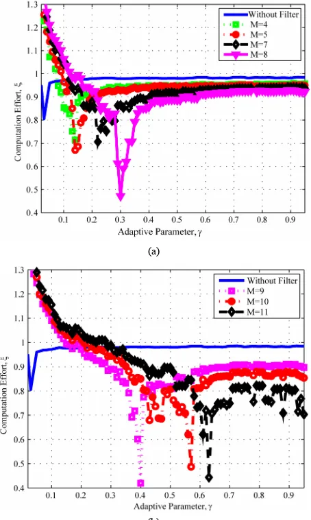
Figure 1 depicts the overall computational effort
for parameter sequences of the type in (14), for different values of . The computational effort was normalized with respect to the overall VI effort to simplify the comparison.
The normalized computational effort for the proposed algorithm is plotted in Figure 1 as a function of the
adaptive parameter . One can see that, for the best
(a)
(b)
Figure 1. Computational effort: Poisson distribution. (a) filter orders M = 4, 5, 7, and 8; (b) filter orders M = 9, 10, and 11.
possible choice of , the computational effort is ap- proximately 0.45 of that of the classical VI algorithm. Therefore, the proposed algorithm converges in about
45% of the time required for the VI algorithm to con- verge. Another point to look at is the improvement due to the moving average digital filter. Five curves are shown in Figure 1(a), the solid blue curve is the overall com-
putational effort without filtering of the empirical rate; the square-marked dotted line curve, the circle-marked dashed line curve, the diamond-marked dashed line curve, and the triangle-marked solid line curve present the com- putational effort with the moving average digital filter defined in (15) of orders M 4,5,7,8, respectively.
This filters are used to process the error sequence ek
prior to the empirical rate estimation in (11). While the unfiltered algorithm produces an improvement over the classic VI algorithm, the use the moving average filter provides an even superior performance, since the filter acts as a smoother of fluctuations in the empirical error function. Moreover, one can see that the performance im- proves as the filter order increases.
Figure 1 also shows that the proposed algorithm is
consistently better than the VI algorithm, for a broad range of parameters . Naturally, a better choice of pa- rameter results in better savings, but the results suggest that the algorithm is robust with respect to the parameter choice. This is a significant improvement over the class of algorithms proposed in [14], which yield more sig- nificant savings in a best-case scenario, but it can be outperformed by VI under a poor parameter selection. Moreover, the algorithm in [14] seems to be overly sen- sitive to the parameter selection and the results tend to vary significantly within a small parameter interval.
One can expect an improvement as the filter order in- creases, up to some point where the increase no longer propitiates an improving performance. This behavior can be observed in Figure 1(b), where the limit is reached
and the best computation effort is achieved with a filter order of M 9, when the algorithm needs about 40%
of the total computation effort.
Figure 2 depicts the computational effort for higher
filter orders, M 12, 13, 15. One can see that no addi-
tional improvement is obtained for orders higher than 9. The main reason is that the underlying process that gen- erates the error sequence ek has a given internal mem-
ory, or process memory. Whenever a estimator, i.e. mov-
ing average filter, exceeds the process memory, the esti- mator will decrease its performance [18].
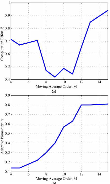
In order to illustrate the impact of the filter order on the computation effort, Figure 3(a) shows the computa-
[image:5.595.60.287.314.693.2]Figure 2. Computational effort: Poisson distribution, filter orders M = 12, 13, and 15.
(a)
(b)
Figure 3. The best adaptive parameter and computation effort as a function of the filter order M for Poisson dis- tribution; (a) computation effort; (b) the best adaptive pa- rameter γ.
Figure 3(b) presents the best adaptive parameter
for different values of filter order. One can notice on
Figure 3(b) that the best value for the adaptive parameter
spans over a wide range. Whenever the filter order is among 8, 9, 10, 11, M
8, 9, 10, 11
, the adaptive pa-rameter has low sensibility, any value of in the range from 0.30 to 0.65, i.e.,
0.30,0.65
, wouldyield a significant improvement in the computational per- formance.
The first experiment suggests that the proposed me- thod can provide significant savings in computational for problems with exogenous Poisson arrival processes. This is a very interesting results considering that such a class of problems tends to be very popular for queueing and manufacturing problems [16,19].
In the second experiment, the clients arrive in the first queue according to a geometric distribution with mean
9
. Clients belonging to the second class arrive uni- formly in the integer interval from 0 to 9. The geometric distribution is also truncated to retain a fraction of 0.9999 of the total transitions and then renormalized. Such a normalization is not needed for the uniform distribution. The joint arrival processes yields 660 possible transitions, hence
x 660 3 1980, .x S
The classical VI algorithm converged in 104 iterations and applied an overall computational effort per state of
5
2.0592 10
[image:6.595.62.287.86.264.2] [image:6.595.61.288.304.684.2] .
Figure 4 depicts the overall computational effort
for parameter sequences of the type in (14), for different values of , normalized with respect to the overall VI effort . For this experiments, we make K20. The
normalized computational effort for the proposed algo- rithm is plotted in Figure 4 as a function of the adaptive
parameter, . One can see that, for a broad range of ,
[image:6.595.310.537.526.702.2]0.01 0.50, the computational effort is less than the classical VI algorithm. At the best point, the cost is about
75% of the classical VI algorithm.
Note that the savings of the proposed algorithm for the second setting, though still appealing, are much less sig- nificant than those obtained for Poisson exogenous arri- val processes. This suggests that more modest savings may be expected for uniform distribution settings. This is consistent with the results in [13], which suggest that PIVI algorithms tend to have a stronger performance for highly concentrated probability distributions, such as the Poisson distribution, while yielding less significant sav- ings for distributions that are widely spread. Moreover, one can also notice that the moving average filter addi- tion seems to have no significant effect on the results.
6. Concluding Remarks
This paper introduced a gradient adaptive version of the partial information value iteration (PIVI) algorithm in- troduced in [13] to the average cost MDP framework, with the addition of a moving average filter to smooth the empirical error sequence.
The proposed algorithm was validated by means of queueing examples, and presented consistent computa- tional savings with respect to classical value iteration. Moreover, the proposed algorithm yielded consistent improvement over value iteration for a wide range of parameters, thus overcoming a shortcoming of a previous approach [14] that was overly sensitive to the parameter choice.
7. Acknowledgements
This work was partially supported by the Brazilian Na- tional Research Council-CNPq, under Grant No. 302716/ 2011-4.
REFERENCES
[1] M. L. Puterman, “Markov Decision Processes: Discrete Stochastic Dynamic Programming,” John Wiley & Sons, New York, 1994.
[2] R. Bellman, “Dynamic Programming,” Princeton Univer- sity Press, Princeton, 1957.
[3] R. Howard, “Dynamic Probabilistic Systems,” John Wil- ey & Sons, New York, 1971.
[4] A. S. Adeyefa and M. K. Luhandjula, “Multiobjective Stochastic Linear Programming: An Overview,” Ameri- can Journal of Operational Research, Vol. 1, No. 4, 2011,
pp. 203-213. [5] M. He, L. Zhao and W. B. Powell, “Approximate Dy-
namic Programming Algorithms for Optimal Dosage De- cisions in Controlled Ovarian Hyperstimulation,” Euro- pean Journal of Operational Research, Vol. 222, 2012,
pp. 328-340 [6] S. A. Tarim, M. K. Dogru, U. Ozen and R. Rossi, “An
Efficient Computational Method for a Stochastic Dy- namic Lot-Sizing Problem under Service-Level Constraints,”
European Journal of Operational Research, Vol. 215, No.
3, 2011, pp. 563-571.
[7] E. F. Arruda, M. Fragoso and J. do Val, “Approximate Dynamic Programming via Direct Search in the Space of Value Function Approximations,” European Journal of Operational Research, Vol. 211, No. 2, 2011, pp. 343-
[8] A. Saure, J. Patrick, S. Tyldesley and M. L. Puterman, “Dynamic Multi-Appointment Patient Scheduling for Ra- diation Therapy,” European Journal of Operational Re- search, Vol. 223, No. 2, 2012, pp. 573-584.
[9] T. Hao, Z. Lei and A. Tamio, “Optimization of a Special Case of Continuous-Time Markov Decision Processes with Compact Action Set,” European Journal of Opera- tional Research, Vol. 187, No. 1, 2008, pp. 113-119.
[10] H. Wang, “Retrospective Optimization of Mixed-Integer Stochastic Systems Using Dynamic Simplex Linear In- terpolation,” European Journal of Operational Research, Vol. 217, No. 1, 2012, pp. 141-148.
[11] P. Benchimol, G. Desaulniers and J. Desrosiers, “Stabi- lized Dynamic Constraint Aggregation for Solving Set Partitioning Problems,” European Journal of Operational Research, Vol. 223, No. 2, 2012, pp. 360-371.
[12] S. D. Patek, “Policy Iteration Type Algorithms for Re- current State Markov Decision Processes,” Computers & Operations Research, Vol. 31, No. 14, 2004, pp. 2333- 2347. [13] A. Almudevar and E. F. Arruda, “Optimal Approximation
Schedules for a Class of Iterative Algorithms, with an Application to Multigrid Value Iteration,” IEEE Transac- tions on Automatic Control, Vol. 27, No. 12, 2012, pp.
[14] E. F. Arruda, F. Ourique and A. Almudevar, “Toward an Optimized Value Iteration Algorithm for Average Cost Markov Decision Processes,” Proceedings of the 49th IEEE International Conference on Decision and Control, Atlanta, 15-17 December 2010, pp. 930-934.
[15] D. M. John and G. Proakis, “Digital Signal Processing,” 4th Edition, Prentice Hall, Upper Saddle River, 2006. [16] P. Brémaud, “Gibbs Fields, Monte Carlo Simulation, and
Queues,” Springer-Verlag, New York, 1999.
[17] D. P. Bertsekas, “Dynamic Programming and Optimal Control,” 2nd Edition, Athena Scientific, Belmont, 1995. [18] R. A. D. Peter and J. Brockwell, “Time Series: Theory
and Methods,” 2nd Edition, Springer, New York, 1991. [19] S. M. Ross, “Stochastic Processes,” 2nd Edition, John Wiley