Munich Personal RePEc Archive
Capital misallocation and aggregate
factor productivity
Azariadis, Costas and Kaas, Leo
Washington University in St. Louis, University of Konstanz
15 June 2009
Capital Misallocation and Aggregate Factor
Productivity
∗
Costas Azariadis
†Leo Kaas
‡June 15, 2009
Abstract
We propose a sectoral–shift theory of aggregate factor productivity for a class of economies with AK technologies, limited loan enforcement, a con-stant production possibilities frontier, and finitely many sectors producing the same good. Both the growth rate and total factor productivity in these economies respond to random and persistent endogenous fluctuations in the sectoral distribution of physical capital which, in turn, responds to persis-tent and reversible exogenous shifts in relative sector productivities. Surplus capital from less productive sectors is lent to more productive ones in the form of secured collateral loans, as in Kiyotaki–Moore (1997), and also as unsecured reputational loans suggested in Bulow–Rogoff (1989). Endogenous debt limits slow down capital reallocation, preventing the equalization of risk– adjusted equity yields across sectors. Economy–wide factor productivity and the aggregate growth rate are both negatively correlated with the dispersion of sectoral rates of return, sectoral TFP and sectoral growth rates. If sec-tor productivities follow a symmetric two–state Markov process, many of our economies converge to a limit cycle alternating between mild expansions and abrupt contractions. We also find highly periodic and volatile limit cycles in economies with small amounts of collateral.
JEL classification: D90, E32, O47
Keywords: TFP, misallocation, sectoral shocks, collateral, reputation
∗We thank Carlos Garriga, Michele Boldrin and seminar participants in Aix–Marseille, Ams-terdam, Athens (AUEB), Carbondale (SIU), Kyoto, Milwaukee (UW), Munich, Rome (Luiss and EIEF), Strasbourg, at the IMF and at the Federal Reserve Banks of Philadelphia and St. Louis for many valuable comments. Leo Kaas thanks the German Research Foundation (grant No. KA 1519/3) for financial support and the Federal Reserve Bank of St. Louis for financial support and hospitality. Costas Azariadis thanks Louiss and Ente Enaudi for their hospitality.
†Department of Economics, Washington University, St. Louis MO 63130-4899, USA. E-mail: [email protected]
1
Introduction
National income accounting exercises conducted by Klenow and Rodriguez-Clare (1997), Hall and Jones (1999) and Chari, Kehoe, and McGrattan (2007) unanimously conclude that total factor productivity is of cardinal importance for both long-run growth and business cycles, including economic depressions. Klenow and Rodriguez-Clare, for example, find that at least 50% of the variation in output per worker in a sample of over 40 countries is attributable to differences in TFP. There is less agreement about the source of productivity differentials. Suggestions range widely from differences in broadly defined social infrastructure advocated by Hall and Jones, to technology adoption barriers proposed by Parente and Prescott (1999), to the labor market frictions studied in Lagos (2006).
This paper is a theoretical investigation of how credit market frictions limit cap-ital mobility and slow down the movement of resources from temporarily less to temporarily more productive sectors, and more generally, from temporarily low to temporarily high valuations. We are pushed in this direction by much evidence con-necting poor economic performance with capital misallocation. Chari et al. (2007) find that financial frictions, defined as “efficiency wedges” which distort the alloca-tion of intermediate inputs among firms,1 account for 60-80% of the US output drop
in the 1929-1933 depression and the 1979-1982 recession, and also for 73% of the variance in detrended U.S. output from 1959 to 2004. Eisfeldt and Rampini (2006) point out that capital reallocation among U.S. firms–defined as sales and acquisition of property, plant and equipment–makes up nearly 25% of total investment on aver-age. Finally, there are strong indications that macroeconomic volatility is connected with the dispersion of both sectoral productivities and sectoral rates of return on capital.2
1
Intermediate inputs are misallocated because they are purchased on credit by producers who face different borrowing costs. Interestingly, Chari et al. find very little explanatory power in “investment wedges”, that is, in time–varying distortions to the economy–wide cost of capital.
2
Lilien (1982) was an early advocate of the importance of sectoral shocks for overall economic activity in an empirical study that connected the aggregate unemployment rate with the cross-sectional dispersion of sectoral employment. More recently, Phe-lan and Trejos (2000) argue in a model with labor–search frictions that sectoral reallocations are quantitatively important for business cycle dynamics. This paper puts Lilien’s idea to work in a growth model with financial frictions and looks at the consequences for productivity and capital accumulation. It is this emphasis on sectoral shocks and productivity which separates our work from earlier literature on financial frictions as a cause of macroeconomic volatility.3
We describe sectoral shifts as idiosyncratic technology shocks in a class of simple economies populated by identical infinitely-lived households and consisting of finitely many sectors that produce the same consumption good. Capital is the only input in production which means that we focus on the misallocation of investment and ignore potentially larger problems stemming from imperfectly functioning labor markets. Sectoral technologies are assumed to be AK with random idiosyncratic productivities and a constant aggregate production possibility frontier, that is, a fixed value for the maximal idiosyncratic productivity. We ignore declining and expanding industries, assuming instead that all sectoral shocks are temporary and reversible.
An ideal economy of this type without any financial frictions would exploit its un-changing aggregate production possiblities to the fullest by moving all physical capital instantly to the most productive sector, and delivering to its population a constantly growing stream of aggregate output and individual consumption. In what follows, surplus capital from less productive sectors is in the form of collateral loans, as suggested by Kiyotaki and Moore (1997), secured by an exogenous fraction
λ ∈ [0,1] of the borrower’s total resources, and also in the form unsecured reputa-tional loans, as in Bulow and Rogoff (1989), which punish defaulters with perpetual exclusion from future borrowing. Both types of loans require endogenous debt limits which rule out default when asset markets are complete. When these limits bind,
in a sample of 40 countries.
3
they slow down capital reallocation and prevent rates of return on capital from reaching equality across all sectors.
Generous debt limits are typical outcomes for economies with abundant collateral, that is, a relatively high value of λ, and with a shared belief among debtors that substantial lines of unsecured credit will continue to be available in the future. Any deterioration in the amount of collateral or in the expected flow of future unsecured credit will tighten current debt limits and impede the flow of capital from lower to higher valuations.
Low capital mobility tends to spell trouble in the class of economies studied in this paper. At one extreme, high values of the collateral parameter λ guarantee perfect capital mobility which, in turn, ensures a unique, rapid and socially desirable balanced growth path. At the other extreme, complete financial autarky, that is, a combination of no collateral and no unsecured lending, leads to macroeconomic disaster. The unique outcome in this case is slow, inefficient and highly volatile growth with strong history dependence.
In between the two extremes of perfect mobility and no mobility lie the relevant cases of modest collateral and unsecured lending. Secured lending by itself tends to generate periodic limit cycles as the distribution of equity shifts in response to persistent changes in relative factor productivities. TFP and the aggregate growth rate do well when most equity is “in the right hands” of highly productive firms, less well when most equity is owned by low–productivity firms. Lower values of the collateral parameter λ typically reduce the average growth rate, increase its dispersion and raise the periodicity of the limit cycle.
The rest of the paper is organized as follows. The next section gives a dramatized preview of results by contrasting an economy of perfect capital mobility with the the worst-case scenario of financial autarky or zero capital mobility. Section 3 de-scribes a more general class of economies with financial frictions. Stationary Markov equilibria are defined in Section 4 and described in Section 5 for economies with se-cured loans only. Section 6 looks at the dynamics of lending when both sese-cured and unsecured loans are traded. Section 7 presents some numerical examples con-necting macroeconomic aggregates with collateral availability and sectoral shocks. Extensions are discussed in Section 8 and conclusions are summarized in Section 9.
2
An Example: Financial Autarky
As a first step towards understanding the importance of financial markets for ag-gregate factor productivity, consider a simple stochastic AK economy which is a special case of the more general model discussed in subsequent sections. There are two sectors i= 1,2, each represented by an infinitely–lived producer with logarith-mic utility of consumption and common discount factor β. Both sectors produce the same consumption/investment good by means of linear technologies with time– varying capital productivity. There are two aggregate states of the world (s = 1,2) with transition probabilities
π(s+|s) =
(
π∈[0,1] if s+ =s ,
1−π if s+ 6=s .
The representative producer in sectorihas access to a linear technology transforming capital input into output with sectoral productivity
Ais =
(
A >0 if i=s , zA if i6=s ,
At the other extreme to frictionless financial markets stands the scenario of financial autarky. Here output growth depends critically on the distribution of wealth between sectors. We denote byx∈[0,1] the wealth share of the productive sector, by (Y, K) the vector of current aggregate output and capital, and by (Y+, K+) the future value
of that vector.
Aggregate output and future capital satisfy
Y =AK[x+z(1−x)], K+ =βY. (1)
The future value of the wealth share x+ equals the ratio of the efficient producer’s
capital tomorrow divided by the future value of aggregate capital K+. This yields
the following stochastic law of motion for the wealth share
x+=
(
f(x;z) ≡ x/[x+z(1−x)] w. prob. π ,
1−f(x;z) = z(1−x)/[x+z(1−x)] w. prob. 1−π . (2)
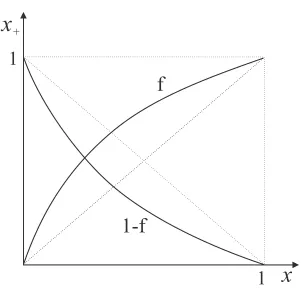
Equation (2) is graphed in Figure 1. From equation (1), we conclude that aggregate factor productivity:
• includes a correction x+z(1−x)<1 due to financial frictions;
• is lower when sectoral productivities are more dispersed, that is, for small values ofz; and
• fluctuates in response to changes in the distribution of wealth between po-tential “borrowers” and “lenders”, that is, between more productive and less productive sectors.
It is easy to check that the aggregate growth rate
Y+/Y =βA[z+ (1−z)x+]
x
1
1
x
+
f
[image:8.612.155.458.81.369.2]1-f
Figure 1: Transition maps for the wealth share under financial autarky.
From the viewpoint of economic theory, the most interesting feature of the law of motion in equation (2) is what it says about the stochastic process of macroeconomic aggregates (factor productivity, the distribution of wealth and the rate of growth) in an economy with no credit market and no capital mobility. All of these stochastic processes turn out to be complex, as one may guess from Figure 1; they visit a countable infinity of states and attain no ergodic distribution. The following result is proved in the Appendix.
Proposition 1: Let π∈(0,1).
(a) For any initial valuex0 ∈(0,1), the wealth share variable xt is a Markov chain on the countably infinite asymptotic set
n
f(x0;zn), f(1−x0;zn)
n∈Z
o
,
(b) The dynamics of aggregate growth and total factor productivity are not ergodic.
This result stands in stark contrast to the equilibrium outcome of the corresponding economy with perfect capital mobility where factor productivity and aggregate out-put growth are constant. We turn now to a more general environment with active asset markets.
3
The environment
Consider a growth model in discrete time t = 0,1,2, . . . with a finite number of agent types (sectors) indexed i∈ I ={1,2, . . . , I} and productivity states s∈ S =
{1,2, . . . , S}. Each sector comprises a continuum of agents with equal size. All agents produce the same good which is available for consumption and investment purposes. Their common preferences over consumption streams are represented by an additively separable expected utility function
E0(1−β)
∞
X
t=0
βtln[c(st)] ,
where st = (s
t, . . . , s0)∈ S1+t is the state history in period t, and the initial state
s0 is given. The productivity state follows a Markov process with transition
prob-ability from s to s+ equal to π(s+|s). In state s an agent of type i can convert
capital into gross output (“resources”) with linear technologyy=Ai
sk. Resourcesy
include current output and undepreciated capital which can be costlessly converted into the single consumption/investment good in the next period. In particular, cap-ital investment is not producer–specific. The simplification that all agents produce the same good isolates the impact of sectoral shocks on capital reallocation while abstracting from relative price effects.
We assume that the economy’s production possibility frontier is constant at A ≡
maxi∈IAis for all s ∈ S. Though we do not need to impose that agent types are
(A1) Every agent operates the technological frontier sometimes; that is, for each i
there exists s such that Ai s=A.
(A2) Not more than one agent type operates the technological frontier; that is, for eachs there is exactly one i such that Ai
s =A.
(A3) No state is trivial; that is, everys∈ S is in the support of the unique invariant state distribution.
Throughout this paper we focus on stationary Markov equilibria where all endoge-nous variables depend only on the current state vector of the economy, denoted
σ ≡ (x, s) ∈ Σ ≡ [0,1]I × S, where x = (x1, . . . , xI) is the distribution of wealth
shares across agent types.
Each period, the less productive agents lend out capital to the more productive agents at the gross interest rateR(σ) that prevails in the credit market. An exoge-nous fraction λ ∈ [0,1] of each agent’s resources is pledgeable collateral which can be seized by creditors in the event of default. The value of λ is constant and com-mon for all producers; it depends on technological factors like the collaterizability of income and wealth, as well as on creditor rights and other aspects of economic institutions.4 Timing within each period is as follows. First the productivity state
is realized; second the credit market opens and agents decide about consumption, investment, borrowing and lending; third, agents produce, borrowers redeem their debt, and everyone carries their wealth into the next period.
Borrowers may choose to default at the end of the period. Any agent who does so loses the collateral share of his resources to creditors and is banned from any unsecured borrowing in all future periods. A defaulting agent is still allowed to lend, however, and also retains full access to secured loans. Since no uncertainty is resolved during debt contracts (that is, borrowing and debt redemption happen within the same period), there exist default–deterring debt limits, defined similarly as in the pure–exchange model of Alvarez and Jermann (2000). These limits are the highest values of debt that will prevent default. In the absence of collateral
4
If resources are split into output and undepreciated capital according toy=Ak= ˜Ak+(1−δ)k, a more general expression for collateral would beλ0Ak˜ +λ1(1−δ)k. Our simplifying assumption
(λ = 0), our enforcement mechanism resembles the one discussed by Bulow and Rogoff (1989) and Hellwig and Lorenzoni (2008) who consider unsecured loans and assume that defaulters are denied excess to future loans but are still allowed to accumulate assets. With λ > 0, secured borrowing is feasible and sometimes, but not always, borrowing limits go beyond an agent’s collateral capacity and sustain a higher flow of credit. Borrowing above one’s collateral is anunsecured loan founded on a producer’s desire to maintain a record of solvency and of continued access to future unsecured loans.
We denote the endogenous constraint on borrower i’s debt–equity ratio by θi(σ).
Whenever the cost of capital R(σ) is strictly below borrower i’s marginal product
Ai
s, this producer will borrow up to his debt limit, and the leveraged equity return
will be ˜Ri(σ) =Ai
s+θi(σ)[Ais−R(σ)]. On the other hand, if agent i’s productivity
is below or equal to the capital yield R(σ), this agent’s equity return is simply ˜
Ri(σ) =R(σ). A defaulting agent, who has only access to secured (collateral) loans,
faces a maximal debt–equity ratioθi
c(σ) =λAis/[R(σ)−λAis], and his equity return is
˜
Ri
c(σ) =AisR(σ)(1−λ)/[R(σ)−λAis] whenR(σ)< Ais, and ˜Ric(σ) =R(σ) otherwise.
It is worth noting that intra–period credit is the only traded asset in this economy. If agents were to trade insurance or contingent claims against next period’s produc-tivity state, these security markets would not open. This immediately follows from the observation that every agent’s marginal utility of wealth ω is proportional to 1/ω, regardless of the agent’s productivity state, so all agents’ security demands are proportional to their wealth. That in turn implies that trade of insurance securities must be zero in equilibrium. We also do not consider a stock market distinct from the loan market. In particular, all shares in other agents’ technologies are equivalent to loans and are subject to default.
The assumption of logarithmic utility implies that all agents consume a fraction 1−β
of wealth, and that the expected utility of a productive borrower with end–of–period wealth ω can be expressed in the form ln(ω) +Vi(σ), whereVi(σ) is end–of–period
utility of agent i with unit wealth when the current state is σ = (x, s).5 Similarly, 5
These assertions follow from the observation that agenti’s flow budget constraint takes the form ωi
= ˜Ri (σ)(ωi
−−c i
) whereci
is consumption and ωi (ωi
if agent i had defaulted in this or in some earlier period, his utility is expressed as ln(ω) +Vi
c(σ) if end–of–period wealth is ω and Vci(σ) denotes end–of–period utility
of a unit–wealth agent of typei who has access to secured loans only.
4
Stationary Markov equilibrium
A stationary Markov equilibrium is a list of functions
h
θi(σ), R(σ),R˜i(σ),R˜ic(σ), vi(σ), Xi(σ)i
i∈I,σ∈Σ . (3)
The first four objects on that list are respectively the debt–equity limits on solvent agents, the cost of capital, and the equity returns for solvent and bankrupt agents. The functions vi(σ) = Vi(σ)−Vi
c(σ) define the “penalty of default” for agent i,
that is, the difference between the continuation utilities from solvency and default. Finally, the maps xi
+ =Xi(σ) : Σ → [0,1] connect this period’s state vector (x, s)
with next period’s wealth share for every agenti. Let X= (Xi)
i∈I : Σ→[0,1]I be the collection of these maps.
In equilibrium, debt limits are the largest values that will deter default when any borrower with equity E is indifferent between solvency and default:
lnhR˜i(σ)Ei+Vi(σ) = lnh(1−λ)Ai
s[1 +θi(σ)]E
i
+Vi c(σ).
Here, the right–hand side is expected utility of the defaulting agent i who leaves the default period with unpledged wealth (1−λ)Ai
s[1 +θi(σ)]E. This equality is
conveniently equivalent to
θi(σ) = (e
vi(σ)
−1 +λ)Ai s
(1−λ)Ais−evi(σ)[Ais−R(σ)] . (4) Equation (4) shows that the maximum default–free debt–equity ratio is increasing in the penalty of defaultvi(σ) and in the collateral share λ. Debt–equity ratios are
also decreasing in the interest rate, and equation (4) gives a lower bound on the equilibrium interest rate: the debt-equity ratio of borroweri tends to infinity when
R(σ) approachesAi
s[1−(1−λ)e−v
i(σ)
Equation (4) shows that θi(σ) is larger than the secured borrowing limit θi c(σ) =
λAi
s/[R(σ)−λAis] for all positive default penalties vi(σ)>0; it reduces to θci(σ) if
vi(σ) = 0. In the following, we refer to an equilibrium with vi(σ) = 0 for all i ∈ I
and σ ∈ Σ as one of secured borrowing; an equilibrium where vi(σ) >0 for at least
somei∈ I and σ∈Σ has secured and unsecured borrowing: here debt–equity limits are based on collateraland reputation.
With aggregate capital K, agent i’s equity is xiK. The supply of credit comes
from all agents with productivity Ai
s ≤ R(σ), and because agents with Ais = R(σ)
are indifferent between lending and borrowing at market rate R(σ), the aggregate supply of credit per unit of aggregate capital is a step function, expressed as the correspondence
CS(σ) =
" X
i:Ai s<R(σ)
xi , X
i:Ai s≤R(σ)
xi
#
.
Similarly, the demand for credit per unit of capital is the correspondence
CD(σ) =
" X
i:Ai s>R(σ)
θi(σ)xi , X
i:Ai s≥R(σ)
θi(σ)xi
#
,
and the credit market is in equilibrium if
CS(σ)∩CD(σ)6=∅ . (5)
As we saw earlier, for any interest yieldR(σ), the equity return of agent i is
˜
Ri(σ) = maxnAis+θi(σ)hAis−R(σ)i, R(σ)o , (6)
while the equity return of a producer with access to secured borrowing is
˜
Rci(σ) = maxnA
i
sR(σ)(1−λ)
R(σ)−λAis , R(σ)
o
. (7)
Agent i’s wealth share changes from xi to
xi+ =Xi(σ) = R˜
i(σ)xi
X
j∈I ˜
Rj(σ)xj , σ= (x
1, . . . , xI, s) . (8)
To understand this expression, suppose that total wealth is one unit today; then agent i’s wealth next period is β times the numerator of (8) while total wealth is β
Expected utilities satisfy recursive equations
Vi(x, s) = (1−β) ln(1−β)+β X
s+∈S
π(s+|s)
(
lnhβR˜i[X(x, s), s+]
i
+VihX(x, s), s+
i )
.
(9) Note again that Vi denotes expected utility of solvent agent i with unit wealth.
In the current period, this agent consumes c= 1−β, and so the first term on the right–hand side is the utility of current consumption; the other terms are discounted future payoffs. In the next period, the distribution of wealth changes from x to
x+ = X(x, s) and the productivity state changes from s to s+ with probability
π(s+|s); the agent saves a fraction β of his unit wealth, ending the period with
wealth ω+=βR˜i(x+, s+) and utility ln(ω+) +Vi[x+, s+].
For an agent who has opted for default in some earlier period, the recursive equation in Vi
c is nearly identical to (9); all that changes is that the equity returns ˜Ri are
replaced by the defaulter’s lower returns ˜Ri
c. By subtracting those equations from
(9), we obtain recursive equations in the default penalties vi(σ) = Vi(σ)−Vi c(σ):
vi(x, s) =β X
s+∈S
π(s+|s)
(
lnR˜
i[X(x, s), s
+]
˜
Ric[X(x, s), s+]
+vihX(x, s), s+
i )
. (10)
Definition: A stationary Markov equilibrium is a list of functions specified in (3)
which satisfies equations (4)–(8) and (10) for all σ= (x, s)∈Σ and i∈ I.
In a stationary Markov equilibrium, the state vector σ is also a sufficient statistic for the growth rate that connects aggregate current resources Y with last period’s resources Y−. In particular, current aggregate capital K equals saving βY−, and current resources are the sum of resources across all agent types:
Y = KX
i∈I
xiR˜i(σ)
= βY−
n
R(σ) + X
i:Ai s>R(σ)
[Ais−R(σ)]xi[1 +θi(σ)]o .
The growth factor is
Y Y− =β
n
R(σ) + X
i:Ai s>R(σ)
This expression has an upper boundβA achieved when no capital is misallocated.
Before we analyze stationary Markov equilibria in detail for some special cases, we state two general results. One of them says that an equilibrium with no unsecured borrowing always exists. In particular,
Proposition 2: There exists a unique equilibrium in which all borrowing is secured.
This result generalizes earlier findings by Bulow and Rogoff (1989) and Kehoe and Levine (1993) who showed that financial autarky is an equilibrium in economies where all borrowing is unsecured. Indeed, it is easy to check thatvi(σ) = 0 together
with ˜Ri(σ) = ˜Ri
c(σ) and θi(σ) = θci(σ) satisfy all equilibrium equations except
market clearing for any given interest rate R(σ). Existence and uniqueness of the market–clearing interest rate is proven in the appendix.
What is the intuition for the equilibrium without unsecured borrowing? If there are no unsecured loans, there is no penalty of default, and therefore no borrower is permitted to borrow in excess of collateral. And conversely, when debt–equity limits just reflect collateral constraints, a good credit record is worthless because there is no default penalty. Section 5 characterizes the secured borrowing equilibrium completely for a symmetric economy with two agent types and two states.
Our second result says that a first–best allocation can only be an equilibrium if there is enough collateral. Specifically, λ ≥ (I −1)/I is a necessary and sufficient condition to support the first best with secured borrowing at the symmetric initial wealth distribution xi = 1/I, i ∈ I. Here returns are equalized, ˜Ri = A, and
the secured borrowing constraint is large enough to shift all capital to the most productive sector in every state.
Can the first best also be supported by secured and unsecured borrowing when
In turn, every borrower would default on an unsecured loan, no matter how small it is. These findings are summed up in
Proposition 3: When λ ≥ (I − 1)/I, the secured–borrowing equilibrium gives rise to a first best allocation for some initial distribution of wealth. Conversely, when λ < (I −1)/I, no first best allocation can be an equilibrium with secured and unsecured borrowing.
The inequalityλ≥(I−1)/Iis stringent, requiring collateral to be a large proportion of available resources, that is, gross national product plus undepreciated capital. In spite of Proposition 3, we will see in Section 6 that unsecured borrowing can still sometimes support production–efficient allocations, particularly in economies with very patient agents and large productivity differences between sectors.
To explore equilibrium with binding constraints in more detail, we focus for the remainder of this paper on the symmetric two–agent, two–state special case of our general environment. In particular, Ai
s = A if i =s, and Asi = zA if i6= s, for i ∈
5
Secured borrowing
In the equilibrium with secured borrowing the debt–equity ratio isθ =λA/[R−λA] and the market–clearing loan yield can be readily obtained as
R(x) =
zA if x≤1−λz , λA
1−x if x∈[1− λz ,1−λ] , A if x≥1−λ .
When borrower wealth is below 1−λ/z, credit demand is so low that the equilibrium interest rate makes unproductive lenders indifferent between production and lend-ing. The economy is production inefficientbecause it misallocates its capital stock. When borrower wealth exceeds this threshold, all capital flows to the more produc-tive agents and the economy becomes production efficient. Forx <1−λ, borrowers are still debt constrained and enjoy a higher equity yield than do lenders. Consump-tion growth rates are higher for borrowers which makes the economy consumption inefficient. Full efficiency in period t is attained only when borrower wealth ex-ceeds 1−λ. In what follows, we assume throughout thatλ < z so that production inefficiency remains a possibility.
The transitional dynamics of borrower wealth is described by two maps. Next period’s borrower wealth is x+ = X0(x) when the productivity state is unaltered
and it is x+ = X1(x) = 1−X0(x) when the productivity state changes. Using
the above expressions for R(x), θ(x) =λA/[R(x)−λA], and the borrowers’ equity return ˜R(x) =A+θ(x)[A−R(x)], we obtain
X0(x) =
˜
R(x)x
˜
R(x)x+R(x)(1−x) =
(1−λ)x
(1−z)x+z−λ , x≤1− λz ,
1−λ , x∈[1−λz ,1−λ] , x , x≥1−λ .
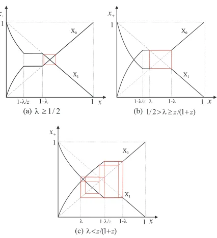
Figure 2 shows the two maps X0 and X1 in three generic situations. It becomes
Proposition 4: In the equilibrium with secured borrowing and for any π ∈ (0,1)
and λ > 0, the dynamics of wealth xt enters a finite stochastic cycle (xn)Nn=1, with
probability one as t→ ∞. The cycle has the following features.
(a) Economies with ample collateral λ ≥ 1/2 converge to a cycle with two states
x2 = 1−x1 ∈[1−λ, λ]. Production is efficient, debt constraints do not bind,
and aggregate output and individual consumption grow at the constant rateβA.
(b) Economies with medium collateral λ ∈[z/(1 +z),1/2) also converge to a cycle with two states and x1 = λ < x2 = 1−λ. Production is again efficient and
aggregate growth is constant at βA. However, individual consumption and wealth growth rates are volatile, and borrowers are constrained in a fraction
1−π of periods. Specifically, agent i’s consumption growth in state st is βA if st=st−1, βAλ/(1−λ) if i6=st 6=st−1, and βA(1−λ)/λ if i=st6=st−1.
(c) Economies with small collateral λ < 1 +z z converge to a cycle with generically
N = 2m states, with m ≥ 2. In 2m −3 of these states, aggregate growth is lower than βA. Cycles are typically asymmetric with booms lasting longer than recessions. The number of states is a weakly decreasing function of λ, and m→ ∞ as λ→0.
Figure 2 illustrates the three possibilities stated in the proposition. In (a), the typical first–best equilibrium is a cycle where borrower wealth fluctuates between two states which means that every agent’s wealth share is constant. Any initial wealth distribution must enter such a cycle with probability one in finitely many periods. In (b), the stochastic cycle again has only two states, but now one of them has constrained borrowers; no capital is misallocated and production is efficient in all periods. And graph (c) shows an example of a cycle with six states, with no misallocation of capital in three of them, and some misallocation in the other three. The red lines indicate the possible transitions between these states.
Figure 2: Asymptotic cycles with secured borrowing.
and dispersed distribution of growth rates around trend. In fact, in the limit where
6
Secured and unsecured borrowing
Equilibria with unsecured borrowing are not easy to describe analytically in any degree of generality. Nonetheless, it is possible to derive a few insightful results for some special cases where the asymptotic wealth dynamics settles down to a finite state space. One such case is the deterministic economy (π = 0), the other is an economy permitting simple production–efficient stochastic cycles with two states. We explore these simpler equilibria in this section.
The deterministic economy admits a steady state with binding constraints where borrower wealth is stable at somex. The wealth share of either type thus periodically alternates between x and 1−x. This is in stark contrast to the stochastic economy where equilibria are typically cyclical and the only possible steady state is a first best outcome with unconstrained borrowers achievable only ifλ ≥1/2. Forλ <1/2, borrower wealth must fluctuate permanently in a stochastic economy.
One obvious steady state in the deterministic model is the one without unsecured borrowing. Although Proposition 4 requires π > 0, it is straightforward to extend the result to the deterministic case as follows. The deterministic economy has a unique steady state x with secured borrowing which is (i) first best when λ ≥1/2; (ii) production efficient and consumption inefficient when z/(1 +z)≤λ <1/2; and (iii) production inefficient when λ < z/(1 +z). In Figure 2 these steady states are at the intersection of the 45o line with the map X
1(.).
For a deterministic economy with secured and unsecured borrowing, we prove the following result in the Appendix.6
Proposition 5: Let π= 0. Then there is a threshold value λˆ≤ z−β2
1−β2 such that
(a) If β ≤ z, there is one steady state with secured borrowing and no steady state with secured and unsecured borrowing.
(b) If β > z and λ ∈[ˆλ,1 +ββ), there is a steady state with secured and unsecured borrowing which coexists with the steady state with secured borrowing.
6
(c) If β > z > β2 andλ ∈(ˆλ,z−β2
1−β2), there is a third steady state with secured and
unsecured borrowing which coexists with the two other steady states of (b).
To interpret these results, the inequalityβ ≤zsimply says that the gains from credit market participation are not high enough to support an equilibrium with unsecured borrowing. Part (a) extends the well–known result of Kehoe and Levine (1993) that intertemporal financial autarky or, in our setting, secured borrowing is the only equi-librium when agents are too impatient or when income fluctuations are too small. Conversely, says part (b), whenβ > z unsecured borrowing is feasible but now col-lateral may not exceed the thresholdβ/(1 +β). If the collateral value is larger than that number, the gain from borrowing above collateral is too small to prevent bor-rowers from defaulting. Put differently, secured borrowing alone supports efficient allocations with low leverage, so that extended credit limits add very little value. Part (c) establishes a strong form of equilibrium multiplicity. In these situations, one steady state turns out to be production efficient whereas the other two steady states are production inefficient. The explanation for equilibrium multiplicity is a
dynamic complementarityin the endogenous borrowing limits. Borrowers’ expecta-tions of future credit market conditions affect their incentives to default today, and this in turn takes an impact on their currentborrowing limits. If future constraints are tight, the payoff from solvency is modest; agents place a low value on the strat-egy of participating in credit markets, and their default penalty is low. In this case, current default–deterring debt limits must be low. Conversely, expectations of loose constraints in the future make participation more valuable, lessen default incentives and ease current constraints.
When agents are sufficiently patient, so that z ≤ β2, the assumptions in part (c)
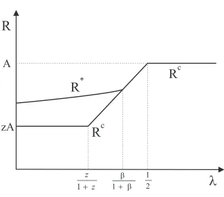
are not valid. Then the deterministic economy has a unique steady state with secured and unsecured borrowing, coexisting with the inferior steady state without unsecured borrowing. Figure 3 shows how steady–state loan yields vary with the collateral parameter λ when z ≤β2.
Figure 3: Steady state loan yields with secured borrowing (Rc) and with secured
and unsecured borrowing (R∗) when z < β2.
locally indeterminate. In particular, there is a continuum of dynamic equilibria in which the value of unsecured loans vanishes asymptotically. Again, this result is explained by the dynamic complementarity between endogenous credit constraints which may trigger a self–fulfilling collapse of the market for unsecured loans: when market participants expect credit constraints to tighten rapidly, the value of repu-tation would shrink over time until only secured loans are traded. Such equilibria are mathematically similar to hyperinflationary equilibria in overlapping–generation models of fiat money but do not require the existence of an unproductive financial asset.
Proposition 6: Let z < β2 and λ < β/(1 +β).
Par-ticularly, there is a continuum of equilibria (θt, xt) such that θt → θc and xt converges to a cycle with period two around xc.
(b) The steady state with secured and unsecured borrowing is locally determinate.
The stochastic economy cannot have a steady state unless it is the first best, and cycles with unsecured borrowing are too complex to describe analytically. Numeri-cally we find that the qualitative features of the transition maps for borrower wealth are much like the ones shown in Figure 2, with the only difference that the cycles do not have finite support, as they do in Figure 2(c).
However, there are still situations where the economy has a stochastic cycle of order two which is production efficient, like the one shown in Figure 2(b). Paralleling Proposition 5, what is necessary for such cycles is that z is small relative to β: agents must be patient enough and their productivity must fluctuate sufficiently so that exclusion from unsecured borrowing is a severe enough punishment. In fact, production–efficient cycles may even exist when there is no collateral at all. The Appendix gives more details about production–efficient cycles.
7
Numerical examples
For a fuller description of stochastic cycles, especially ones that exhibit some misal-location of capital, we use value function iteration to isolate stationary Markov equi-libria with reputational borrowing. Specifically, for arbitrary initial default penalties for agent 1 v1
0(.,1)>0 and v01(.,2)>0,7 we calculate constraints and interest rates
for allxusing the equilibrium conditions (4)–(7) and the wealth iteration maps (8). The results are then substituted in the right–hand side of (10) to calculate new default penaltiesv1
1(.,1) andv11(.,2), and so on. Our previous results on equilibrium
multiplicity imply that this map cannot be a global contraction, so one cannot expect a definitive proof that equilibrium exists. We find, however, that these iterations converge fast, and we are able to identify the theoretical equilibria in the special
7
Because of symmetry, default penalties for agent 2 are simplyv2
(x,1) =v1
(x,2) andv2
(x,2) =
v1
cases analyzed in previous sections. We conjecture that the iteration procedure generally converges to the determinate equilibrium whenever there is equilibrium multiplicity. In the deterministic economy π = 0, for example, we know that the secured–borrowing equilibrium is determinate whenever no other equilibrium exists, and indeterminate otherwise (Proposition 6). Numerically we find indeed that value function iteration converges to the determinate equilibrium.
For a plausible benchmark parameterization, we study how aggregate growth and volatility depend on the model parameters and how they qualitatively correlate with the sectoral dispersions of equity returns and total factor productivities. It is not the purpose of this exercise to conduct a full–blown quantitative analysis; that would require a much more detailed model incorporating labor and some other features discussed in the next section. We fix the three parameters A = 1.08,β = 0.96 and
π = 0.9 so that annual growth in the first–best economy is at 3.7% and sectoral productivity shifts are rather persistent with a mean duration of 10 years. We then explore how the features of the economy change when we vary the key parameters
λ and z.
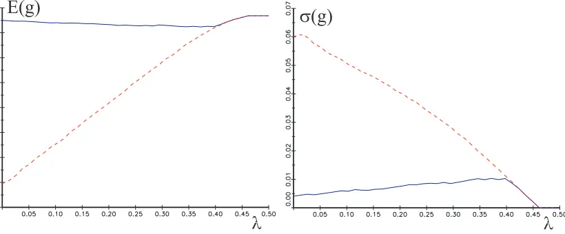
borrow-ing, less collateral makes the potential exclusion from unsecured loans more harmful and thereby relaxes credit limits; hence growth increases slightly and becomes less volatile.
l
l
[image:25.612.102.512.156.326.2]E(g)
s
(g)
Figure 4: Mean and standard deviation of growth as λ varies from 0 to 0.5 where
A = 1.08, β = 0.96, π = 0.9 and z = 0.85. The secured–borrowing equilibrium is shown by the red (dashed) curve, and the equilibrium with secured and unsecured borrowing is blue (solid). E(g) and σ(g) are calculated as sample averages for a time series of 50,000 periods.
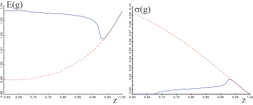
Figure 5 shows the result of a similar simulation when λ is fixed at 0.2 andz varies from 0.6 to 1.0. Clearly, when z is close to one, the economy is almost first best and growth is constant atβA≈1.037. For values of z above 0.94, there is a unique equilibrium with secured borrowing; a second equilibrium with unsecured borrowing emerges for a larger productivity spread between the two sectors. Interestingly, unse-cured borrowing permits a more efficient allocation of capital when the productivity difference between the two sectors is larger. Indeed, the equilibrium with secured and unsecured borrowing achieves a production efficient allocation of resources for values ofz below 0.67.
At the benchmark parameter values with λ = 0.2 and z = 0.85 we also calculate equity return dispersion as the spread between sectoral equity returns, measured by the weighted standard deviation between ˜R1
t and ˜R2t where weights are the
z
z
E(g)
s
[image:26.612.97.513.93.267.2](g)
Figure 5: Mean and standard deviation of growth as z varies from 0.6 to 1 where
A = 1.08, β = 0.96, π = 0.9 and λ = 0.2. The secured–borrowing equilibrium is shown by the red (dashed) curve, and the equilibrium with secured and unsecured borrowing is blue (solid). E(g) and σ(g) are calculated as sample averages for a time series of 50,000 periods.
borrowing, we find that this measure averages around 5.4% and has a standard de-viation of 7%, the same order of magnitude as the stock–market dispersion indices reported in Loungani, Rush, and Tave (1990) (Fig. 1). The correlation coefficient between equity–return dispersion and gt is -0.80, which is in line with the evidence
listed in the introduction. Growth is low when capital is misallocated in which case the dispersion between sectoral equity returns is large. Figure 6 shows time series for the growth rate of aggregate resources and for the dispersion of equity returns for a simulation of 50 periods at the benchmark parameter values.
Figure 6: Simulated equilibrium with secured and unsecured borrowing at parame-ters A = 1.08, β = 0.96, π = 0.9, z = 0.85 and λ = 0.2: Growth rate (solid, blue) and dispersion of equity returns (dashed, red), both as deviations from their mean.
8
Extensions
8.1
Sector–specific labor
The absence of any input from labor is the biggest abstraction in our model, but its impact is quantitative rather than qualitative. A quick remedy, along the lines suggested by Kiyotaki and Moore (2008) and Kocherlakota (2009), would replace our AK technologies with standard neoclassical constant return ones of the form
Y = Ai
sF(Ksi, Nsi). Each sector would be populated with one unit of immobile
labor. Labor will consume its marginal product and all saving would still be done by capitalistsi∈ I who hire labor at a competitive wage wi
s and face a competitive
yield on each unit of capital, that is,
Ris= max
N≥0
n
Finally, pledgeable collateral will be an exogenous fractionλof capital income rather than of all income, and long–term growth can be added by endowing sectoral pro-ductivity shocks with a common trend. We expect this extension to be relatively straightforward provided that labor is completely immobile.
8.2
Irreversible investment
Unsurprisingly, each of the two sectors is considerably more volatile than the aggre-gate economy. Because every stochastic cycle must enter some occasional periods of production efficiency, output in any sector falls occasionally to zero. This circum-stance prevents a meaningful calculation of sector growth rates. Further, it appears to be a strong abstraction to assume that all gross resources can, in the extreme, move between sectors from one period to the next. To deal with these limitations, it seems a sensible extension to augment the model by some sector specificity (invest-ment irreversibility).8 For simplicity, suppose that a constant fraction of resources
is sector specific and cannot be employed in the other sector, and let Ψ<1 be the share of resources which is usable in both sectors. Then the only change to the model is that the expression for credit supply CS(σ) is multiplied by the factor Ψ, and all other equations remain unchanged. It is important to emphasize, however, that now even the first–best economy involves fluctuations of aggregate output, as resources move sluggishly between sectors when the productive state changes.
In the numerical example, suppose that 90 percent of capital is sector specific (Ψ = 0.1). For the benchmark parameter values with λ= 0.2 and z = 0.95, mean growth falls from 2.1% (at Ψ = 1) to 1.4% (at Ψ = .1) whilst its standard deviation increases from 1.3% to 1.9%. The growth rate of either sector, however, has a standard deviation of about 9.6%, five times larger than the standard deviation of aggregate growth. In line with the evidence discussed in the introduction, the dispersion between sector growth rates is countercyclical; its correlation coefficient with aggregate growth is -0.36.
8
8.3
Sectoral comovement
Another feature of the cycles characterized in the previous sections is that growth rates in the two sectors are negatively correlated. As an implication, either one sector is pro–cyclical and the other is counter–cyclical or both sectors are acyclical. The evidence however strongly supports comovement of virtually all two–digit industries with aggregate output (see e.g. Christiano and Fitzgerald (1998)). In the previous example, the absence of comovement is an artefact of the two–sector, two–state specification, where business cycles are exclusively driven by sectoral productivity shifts between two constant productivitiesAandzA. When technologies are in some way correlated with the sectoral productivity shifts, comovement follows easily. This is relatively simple when the technology frontier is volatile, but is also possible with a constant frontier. To see this in an extension of the model which retains perfect symmetry between sectors, suppose that the technology parameter z attains one of two valueszc andzn, depending on whether the sectoral state changes or not. That
is, “change of states” haszt =zc whenst6=st−1, and “no change of states” haszt=
zn whens
t =st−1. This extension thus has two sectors and four productivity states
(st, st−1)∈ {1,2}2. In the numerical example with the same benchmark parameter
values, we find that there is comovement (i.e. positive correlations between aggregate growth and growth rates of each sector) if zc = 0.99 > zn = 0.95 (and Ψ = 0.9).
Alternative mechanisms are possible which can generate comovement for aggregate shocks to A or to the collateral share λ which are correlated with sectoral shifts.
8.4
Other loan enforcement mechanisms
provided that all agents share a commonhigh discount factor and have sufficiently large income variability (see also Azariadis and Kaas (2007)). Similar results can also be obtained for our model; the only change in the model’s equilibrium equations is that the defaulters’ equity returns ˜Ri
c(x, s) in equations (10) must be replaced by
the autarkic returnsAi
s. In the two–agent, two–state special case without collateral,
it is straightforward to show that there is a first–best equilibrium at the symmetric wealth distribution iff
ln 1z ≥ (1−β)(1 +β−2βπ) β(1−π) ln 2 .
Thus the first best is an equilibrium if the productivity differential is sufficiently large or if agents are sufficiently patient.
On the other hand, one can also think ofweakerpunishment scenarios in our model. For example, defaulting agents may be shut out of unsecured credit for a finite number of periods before they regain unlimited access to unsecured loans. Alter-natively, defaulters may sometimes evade punishment and have a positive chance of obtaining unsecured loans. Both mechanisms are rather straightforward exten-sions of our model. Shortened punishment periods and lower detection probabilities tighten debt limits considerably and thereby contribute to lower growth and higher aggregate TFP volatility.
9
Conclusions
This paper outlines a financial theory of aggregate factor productivity which con-nects the sectoral allocation of capital with sectoral productivity shocks and credit market frictions. We emphasize frictions arising from insufficient collateral for se-cured loans and from the limited enforcement of unsese-cured loans. Both of these lead to endogenous debt limits which slow down the reallocation of surplus capital from less productive to more productive sectors, and prevent the equalization of sectoral productivities and sectoral rates of return.
dispersion of sectoral growth rates. If we reinterpret “sectors” to be individual firms, then our results are also consistent with recent work by Hsieh and Klenow (2007) who find that industry productivity dispersion is negatively correlated with industry productivity in a panel that includes data from the U.S., China and India. Alterna-tively, if we index countries by the fraction of collateral assets to total resources, our results are in line with Diebold and Yilmaz (2008) who find that macroeconomic volatility is positively correlated with stock market volatility in a cross section of countries.
A clear example of macroeconomic volatility is the one that, as of this writing, is gripping developed economies throughout the world. Its symptoms are a substantial fall in economic activity and unusually steep reductions in asset prices and the volume of credit. For example, seasonally adjusted weekly averages of all commercial paper issued in the United States fell from $170bn for all of 2007 to just about $100bn for the week ending June 12, 2009. The seasonally adjusted stock of all commercial paper outstanding dropped by 20% in the six months following November 30, 2008.
Our model offers a simple explanation for such episodes of rapid disintermediation. We interpret them as transitions from a well—intermediated, socially desirable and fragile state with plenty of unsecured credit to a poorly–intermediated, less desirable but asymptotically stable state in which all loans are collateralized. The impulse for this transition is widespread skepticism about the ability of financial intermediaries to continue the provision of unsecured credit at the volume needed to support the socially desirable equilibrium. An equivalent interpretation of the movement from the good to the bad state is that it is triggered by a “sunspot” variable, similar to the bubble bursting equilibrium considered by Kocherlakota (2009). We conjecture that bubbles on financial assets are equivalent to unbacked private debt in our environment, as they are in the pure–exchange model of Hellwig and Lorenzoni (2008).
References
Alvarez, F., and U. Jermann (2000): “Efficiency, Equilibrium, and Asset Pric-ing with Risk of Default,” Econometrica, 68, 775–797.
Azariadis, C., andL. Kaas(2007): “Asset Price Fluctuations without Aggregate Shocks,” Journal of Economic Theory, 136, 126–143.
Brainard, S., and D. Cutler (1993): “Sectoral Shifts and Cyclical Unemploy-ment Reconsidered,” Quarterly Journal of Economics, 108, 219–243.
Bulow, J., and K. Rogoff (1989): “Sovereign Debt: Is to Forgive to Forget?,”
American Economic Review, 79, 43–50.
Chari, V., P. Kehoe, and E. McGrattan (2007): “Business Cycle Account-ing,” Econometrica, 75, 781–836.
Christiano, L., and T. Fitzgerald (1998): “The Business Cycle: It’s Still a Puzzle,” Federal Reserve Bank of Chicago Economic Perspectives, 22, 56–83.
Diebold, F., and K. Yilmaz(2008): “Macroeconomic Volatility and Stock Mar-ket Volatility, Worldwide,” NBER Working Paper 14269.
Eisfeldt, A., and A. Rampini (2006): “Capital Reallocation and Liquidity,”
Journal of Monetary Economics, 53, 369–399.
Hall, R., and C. Jones (1999): “Why Do Some Countries Produce So Much More Output Per Worker than Others?,” Quarterly Journal of Economics, 114, 83–116.
Hellwig, C.,and G. Lorenzoni(2008): “Bubbles and Private Liquidity,” NBER Working Paper 12614.
Hsieh, C.-T., and P. Klenow (2007): “Misallocation and Manufacturing Pro-ductivity in China and India,” NBER Working Paper No. 13290.
Kehoe, T., and D. Levine (1993): “Debt–Constrained Asset Markets,” Review of Economic Studies, 60, 865–888.
(2008): “Liquidity, Business Cycles, and Monetary Policy,” Working Paper, Princeton University.
Klenow, P., and A. Rodriguez-Clare (1997): “Economic Growth: A Review Essay,” Journal of Monetary Economics, 40, 597–617.
Kocherlakota, N. (2009): “Bursting Bubbles: Consequences and Cures,” Mimeo, University of Minnesota.
Lagos, R.(2006): “A Model of TFP,”Review of Economic Studies, 73, 983–1007.
Lilien, D. (1982): “Sectoral Shifts and Cyclical Unemployment,” Journal of Po-litical Economy, 90, 777–793.
Loungani, P., M. Rush, and W. Tave (1990): “Stock Market Dispersion and Unemployment,” Journal of Monetary Economics, 25, 367–388.
Matsuyama, K. (2007): “Credit Traps and Credit Cycles,” American Economic Review, 97, 503–516.
Parente, S., and E. Prescott (1999): Barriers to Riches. MIT Press, Cam-bridge, MA.
Phelan, C., and C. Trejos (2000): “The Aggregate Effects of Sectoral Reallo-cations,” Journal of Monetary Economics, 45, 249–268.
Appendix
Proof of Proposition 1:
(a) Let g(x;z) ≡ 1−f(x;z) and define (fn, gn) to be the n–order iterates of the
maps (f, g), where (f0(x;z), g0(x;z)) = (x, x) and (f1, g1) = (f, g). Then one easily
shows
fn(x;z) = f(x;zn) for all n≥0 ,
g2(x;z) = x , g[f(x;z);z] = g(x;z2) ,
for all z ∈ [0,1]. For any initial value x0 ∈ (0,1), we can easily show by induction
that xt is a Markov chain on the asymptotic set
n
x0, f(x0;zn), f(1−x0;zn),1−x0, g(x0;zn), g(1−x0;zn) forn ≥1
o
.
However, x0 = f(x0;zn) for n = 0, 1 −x0 = g(x0;zn) for n = 0. In addition,
g(x;zn) =f(1−x;z−n) for all x and n ≥1. Therefore the set of asymptotic states
consists of the list in Proposition 1 if we allow n to be any integer.
(b) Follows from the fact that the set of asymptotic states depends on the initial
valuex0. ✷
Proof of Proposition 2:
It remains to show existence and uniqueness of a market–clearing interest rateR =
R(σ) with secured borrowing for anyσ = (x, s). For any R > λA≥ λAi
s, collateral
debt limits are θi c(R) =
λAis
R−λAis. Debt limits are decreasing in the interest rate,
and so is the demand for credit CD(σ); it is a downward–sloping function with finitely many upward jumps atR =Ai
s, it is zero at R≥A and it tends to infinity
as R → λA. On the other hand, the supply of credit CS(σ) is a weakly increasing step function which is zero atR= 0 and finite at R≥A. Because of these features, there exists a unique market–clearing interest rate for any σ. ✷
Proof of Proposition 3:
A candidate first–best equilibrium has stable wealth shares x∗ = (xi∗)
i∈I and an interest factor equal to the frontier productivity, R(x∗, s) = A for all s ∈ S. With secured borrowing (vi = 0), the debt limits then follow from (4) as θi(x∗, s) =
λ/(1−λ) for alli∈ I ands∈ S. In every productive states, there is by assumption (A2) a unique agent i(s) using the frontier technology. Because of (A3), no state is trivial, hence credit market equilibrium requires that for any s ∈ S, agent i(s)’s maximum demand for credit does not exhaust credit supply of all other agents:
λ
1−λxi(s)∗ ≥
X
j6=i(s)
xj∗ = 1−xi(s)∗ , s∈ S ,
with secured borrowing iff λ ≥ 1−xi∗ for all i ∈ I. For this to be true at some
distribution of wealthxi∗, it must hold in particular at the symmetric distribution of wealth,xi∗ = 1/I. Therefore, the conditionλ≥(I−1)/I is necessary and sufficient for the first best to be an equilibrium with secured borrowing for some distribution of initial wealth.
Now suppose thatλ < (I−1)/I and suppose that there is a first–best equilibrium with secured and unsecured borrowing at stable wealth distribution x∗ = (xi∗)
i∈I and interest yields R(x∗, s) = A, s ∈ S. But then from (6) and (7), ˜Ri(x∗, s) =
˜
Ri
c(x, s) =A for all i∈ I and s∈ S, and from (10) follows that vi(x∗, s) = 0 for all
(i, s). But this in connection with (4) implies again that all borrowing is secured, so debt limits areθi(x∗, s) =λ/(1−λ), and the credit market cannot be in equilibrium,
as seen above. ✷
Proof of Proposition 4:
Parts (a)–(b) follow simply from inspection of Figure 2 (a) and (b). To prove (c), it is useful to note the following features of the maps X0(x) and X1(x). For any
x≤1−λ/z, it holds that X1X1(x) =x and that X0X1(x) = 1−x.
Again it is clear from the graph that the minimum and maximum elements of the asymptotic invariant set arex=λ and x= 1−λ. Let ℓ≥1 be the unique number such thatXℓ−1
0 (λ)<1−λ/z andX0ℓ(λ)≥1−λ/z and suppose the last inequality is
strict (a generic feature). Obviously then, Xk
0(λ), k = 1, . . . , ℓ are also elements of
the asymptotic invariant set. Further elements are the ℓ wealth statesX1X0k(λ) for
k= 0, . . . , ℓ−1, which are all in the interval (λ,1−λ/z] and which are generically different from the other elements. Note that X1X0ℓ(λ) = λ is not a new element of
the asymptotic invariant set. To see that there are no further elements, note that any further iteration fromX1X0k(λ) can only lead either toX1X1X0k(λ) =X0k(λ) or
to X0X1X0k(λ) = 1−X0k(λ) = X1X0k−1(λ) which are both already elements of the
asymptotic invariant set. Hence the asymptotic invariant set comprises λ, 1 −λ,
Xk
0(λ) for k = 1, . . . , ℓ and X1X0k(λ) for k = 0, . . . , ℓ−1, which are 2ℓ+ 2 = 2m
elements with m = ℓ + 1 ≥ 2. Of these, exactly the three [1 − λ, Xℓ
0(λ) and
X1(λ) = 1−λ/z] are not smaller than the threshold 1−λ/z and have growth rates
Proof of Proposition 5:
Without loss of generality, setA= 1 to simplify notation. Consider first a production– efficient steady statex with debt–equity constraint θ = (1−x)/x and interest rate
R ∈(z,1). x is a steady state if x=X1(x) =R(1−x), and hence x =R/(1 +R),
θ= 1/R, ˜R= 1 +θ(1−R) = 1/R, and ˜Rc =R(1−λ)/(R−λ). Let v andw be the
default penalties for borrowing and lending agents (of both types) in steady state. From (10) follows that v and w satisfy
v = βw , (11)
w = βnlnhR˜˜
Rc
i
+vo . (12)
Hence,
v = β2 1−β2 ln
˜
R
˜
Rc
= β2 1−β2 ln
R−λ R2(1−λ)
.
On the other hand, (4) implies that
v = lnh(1−λ)(1 +R)i . (13)
From these two equations follows that the steady–state interest rate must solve
(1−λ)1/β2R2(1 +R)(1−β2)/β2 =R−λ . (14)
Moreover, unsecured borrowing requires that v > 0 which, from (13), implies that
R > Rc ≡ λ/(1−λ), where Rc is the interest rate with secured borrowing which
is always a solution of equation (14). Another solution R∗ > Rc exists provided
that the slope of the LHS at Rc is smaller than one. This turns out to be the case
if and only if λ < β/(1 +β). Now R∗ indeed constitutes an equilibrium provided that R∗ > z and R∗ <1. The latter inequality follows if LHS>RHS at R = 1. But this turns out to be equivalent toλ < 1/2 which follows from λ < β/(1 +β). The first inequality is true either if Rc ≥ z (which is the same as λ ≥ z/(1 +z)) or if
LHS<RHS at R =z. This last inequality is expressed as
(z−λ)β2 1−λ > z2β
2
(1 +z)1−β2
. (15)
λ0 ≥z/(1 +z) holds, and hence (15) is violated for any λ≤z/(1 +z); hence there
is no steady state with unsecured borrowing in this case. When z < β, there must be a threshold ˜λ < λ0 where (15) holds with equality. Hence, with ˆλ = max(0,˜λ),
there exists a steady state with unsecured borrowing for anyλ∈[ˆλ, β/(1 +β)).
Next consider a production–inefficient steady state where R =z, ˜R = 1 +θ(1−z) and ˜Rc =z(1−λ)/(z−λ), and again let v be the stationary penalty of default for
a borrowing agent. Now (11) and (12) can be expressed as
v = β2 1−β2ln
[1 +θ(1−z)](z −λ)
z(1−λ)
,
and (4) becomes
v = lnh(1−λ)(1 +θ) 1 +θ(1−z)
i
. (16)
Equating the two yields an equation in the debt–equity ratio,
1 +θ =1−λ/z
β2
1−β21 +θ(1−z) 1−λ
1 1
−β2
. (17)
Here, the debt–equity ratio with secured borrowingθc =λ/(z−λ) solves this
equa-tion. Another solutionθ∗ corresponds to an equilibrium with unsecured borrowing only if θ∗ > θc, and such a solution exists iff the slope of the RHS at θc is smaller
than one. This is the case iff
λ < λ0 = z−β 2
1−β2 .
The solution θ∗ > θc indeed gives rise to a production–inefficient equilibrium at
R=z if θ∗ <(1−x∗)/x∗ at the stationary borrower share x∗ which satisfies
x=X1(x) = [1 +θ∗ z(1−x)
(1−z)] +z(1−x) ,
or
(1−z)(1 +θ∗)x2+ 2zx−z = 0 .
Clearly this quadratic has a unique solution x∗ ∈ (0,1) for any θ∗ > 0. Now
is equivalent to (15) again. Because the LHS in (15) is increasing in λ∈[0, λ0], the
inequality is satisfied for all λ∈(ˆλ, λ0). Hence
ˆ
λ < λ < z−β2
1−β2
is a necessary and sufficient condition for a production inefficient steady state equi-librium with secured and unsecured borrowing. ✷
Proof of Proposition 6:
In the deterministic economy, the dynamic versions of the steady–state equations (11) and (12) can be simplified to
vt=β2ln
R˜
t+2
˜
Rtc+2
+β2vt+2 . (18)
Suppose first that the economy is production inefficient in all periods. Then,Rt=z,
˜
Rc
t =z(1−λ)/(z−λ), and from (4) follows
˜
Rt= 1−λ(1−−evλt(1)z−z) .
Substitution into (18) yields
vt =β2ln
z−λ
1−λ−evt+2(1−z)
+β2v
t+2 .
Note thatvt is a forward–looking (jump) variable. Hence, the steady statev = 0 is
locally indeterminate iffdvt/(dvt+2)|v=0 >1. But this condition turns out to be the
same as
λ > z−β2
1−β2 ,
which follows fromz < β2. Hence, there is an infinity of equilibria withv
t →0 (and
thusθt →θc). In the limit, the dynamics of borrower wealth becomes
xt+1 = z(1−−λ+xt)(xz−λ)
t(1−z) =X1(xt),
which satisfies xt+2 = X12(xt) =xt. Hence, in all these equilibria, wealth converges
Next consider a production–efficient economy. Here θt = (1−xt)/xt, and from (4)
follows
Rt= 1−e
−vt(1−λ)
1−xt ,
˜
Rt= 1ev−txλ
t ,
˜
Rct = [1−e
−vt(1−λ)](1−λ)
1−e−vt(1−λ)−λ(1−x
t)
.
Substitution into (18) yields
vt=β2ln
1−e−vt+2(1−λ)−λ(1−x t+2)
[evt+2−1 +λ]x t+2
+β2vt+2 . (19)
The dynamics of borrower wealth is
xt+1 = Rt(1−xt)
Rt(1−xt) + ˜Rtxt
= 1−e−vt(1−λ) .
Substitution into (19) gives
vt =β2ln
1−e−vt+2(1−λ)−λ(1−λ)e−vt+1
[evt+2 −1 +λ][1−e−vt+1(1−λ)]
+β2vt+2 .
Using ϕt=evt, this equation is more conveniently expressed as
ϕt=
ϕt+1(ϕt+2−1 +λ)−λ(1−λ)ϕt+2
(ϕt+2−1 +λ)(ϕt+1−1 +λ)
β2
. (20)
A steady state is a solution of
ϕ(1−β2
)/β2
= ϕ−1 +λ2
(ϕ−1 +λ)2 . (21) One solution is ϕ = 1 which (under appropriate conditions) gives rise to a steady state with secured borrowing. A steady state with secured and unsecured borrowing must be a solution with ϕ >1. Againϕt is a forward–looking jump variable; hence
a steady state is locally determinate if both eigenvalues of the backward dynamics (20) have modulus less than one, and a steady state is locally indeterminate if at least one eigenvalue has modulus larger than one. It is straightforward to calculate the determinant and trace of the Jacobian at the steady state:
D=− dϕt
dϕt+2 =
β2λ(1−λ)2
(ϕ−1 +λ)(ϕ−1 +λ2) ,
T = dϕt
dϕt+1 = −
β2(ϕ−1)(1−λ)2