Cointegration and causality between Romanian exports and imports

Munich Personal RePEc Archive

Cointegration and causality between

Romanian exports and imports

Dumitriu, Ramona and Stefanescu, Razvan and Nistor,

Costel

Dunarea de Jos University of Galati, Dunarea de Jos University of

Galati, Dunarea de Jos University of Galati

3 May 2009

Online at

https://mpra.ub.uni-muenchen.de/42091/

COINTEGRATION AND CAUSALITY BETWEEN

ROMANIAN EXPORTS AND IMPORTS

Ramona DUMITRIU, Razvan STEFANESCU, Costel NISTOR

“Dunarea de Jos” University Galati, Faculty of Economic Sciences [email protected]

Abstract: This paper explores the dynamic relations between the Romanian exports and imports using monthly data from January 2005 to March 2009. We test the cointegration and causality between the two variables. The results of Engle-Granger, Johansen and cointegration tests are ambiguous while the Breitung test infirmed the hypothesis of cointegration between exports and imports. In these circumstances we conclude that we can’t consider Romanian current account deficits as sustainable. We also find evidence of the bidirectional Granger causality between the exports and the imports explained by the significant interactions between the two variables.

Keywords: Causality, Cointegration, Romanian Foreign Trade JEL Classification: F10, F19, F40

1. INTRODUCTION

The analysis of relations between the exports and the imports is an important tool for studying the perspectives of a country foreign trade. In the recent years these relations were investigated by cointegration and causality techniques. Husted (1994) pioneered the use of cointegration techniques in the analysis of the exports and imports convergence in the long-run. Arize (2002) found that a country current account was sustainable if the exports and the imports were cointegrated and the cointegration coefficient was statistically equal to one. The reciprocal influences between the exports and the imports could be studied in a Granger – Causality framework that reveals if the information relevant to the prediction of them is contained solely in the two time series data (Granger 1969).

The study of dynamic relationships between Romanian exports and imports has some particularities provided by the frequently significant changes that occurred in the last years. In these circumstances, in this article we use monthly data from January 2005 to March 2009employing tests of stationarity and cointegration that allow taking into account the structural breaks.

The remaining part of this paper is set out as follows. The second part approaches the data and methodology we employ. The empirical results of the analyses are presented in the third part and the fourth part concludes.

2. DATA AND METHODOLOGY

In this analysis we employ monthly data about the Romanian exports and imports of goods and services transactions provided by National Bank of Romania. Our sample covers the period from January 2005 to March 2009. Because of the significant seasonality of these values we apply the ARIMA (Autoregressive Integrated Moving Average) technique to obtain seasonally adjusted values. We use four variables:

- NEXP for the natural logarithms of seasonally adjusted values of nominal exports of goods and services; - NIMP for the natural logarithms of seasonally adjusted values of nominal imports of goods and services; - d_ NEXP for the first differences of NEXP;

- d_ NIMP for the first differences of NIMP.

We analyze the stationarity of the four time series applying two unit root tests: the classic Augmented Dickey Fuller (1979) and a test proposed by Saikkonen and Lutkepohl (2002) and Lanne et al. (2002) which allows taking into account the structural breaks. For selecting the numbers of lagged differences we use four criteria: Akaike Info Criterion (AIC), Final Prediction Error (FPE), Hannan-Quinn Criterion (HQC) and Schwarz Criterion (SC).

3. EMPIRICAL RESULTS

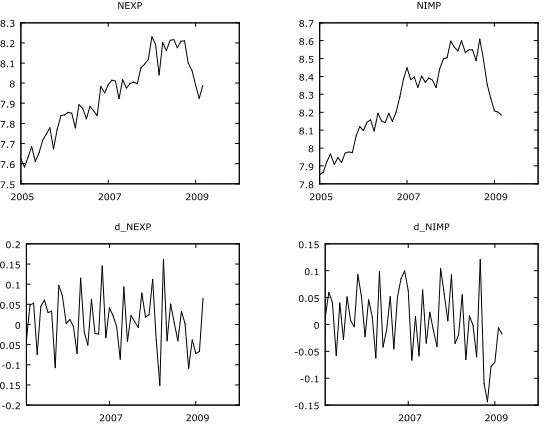
We test the stationarity of exports and importsfor level values and for their first differences. For level values we use intercept and time trend as deterministic terms (see Figure 1).

Fig. 1. Evolution of NEXP and NIMP for the level values and for their first differences

The results of Augmented Dickey Fuller Test, presented in the Table 1, suggest that we cannot rule out, for both NEXP and NIMP, the null hypothesis of a unit root.

Table 1. Augmented Dickey Fuller Unit Root Test for NEXP and NIMP

Variable Lagged differences Test statistics AIC, FPE: 6 -1.0765 NEXP

HQC, SC: 0 -2.2692 AIC, FPE: 4 0.8637 NIMP

HQC, SC: 0 -0.1891

We continue by applying unit root tests with structural breaks for level values. The results presented in the Table 2 indicate again that both variables have unit roots.

Table 2. Unit root tests with structural breaks for NEXP and NIMP

Variable Shift Function Break Date Lagged differences Test statistics 2008 M3 AIC, FPE, HQC: 6 -1.7542 Impulse dummy

2008 M3 SC: 1 -1.7783 2008 M3 AIC, FPE: 3 -1.8302 NEXP

Shift dummy

2008 M3 HQC, SC: 0 -2.4104 Impulse dummy 2008 M9 AIC, FPE, HQC, SC: 0 -1.1329 2008 M11 AIC, FPE, HQC: 3 -2.1579 NIMP

Shift dummy

Based on the graphical representation we use, for the first differences values only intercept as deterministic term. The results of Augmented Dickey Fuller Test, presented in the Table 3, suggest that both d_NEXP and d_NIMP are stationary time series.

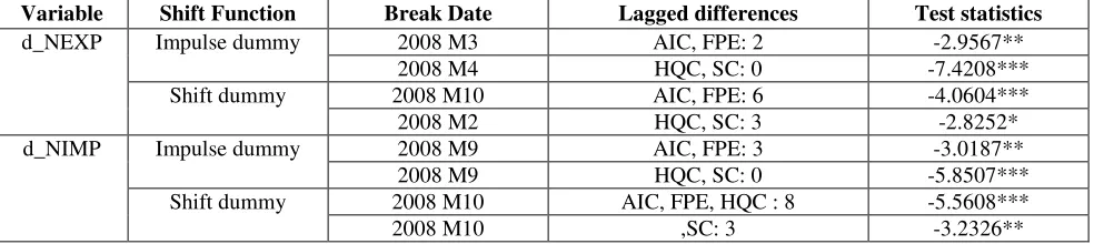
We also analyze the stationarity of the first differences values of the two variables using unit root tests with structural breaks. The results presented in the Table 4 indicate that we can reject, for both time series, the null hypothesis of a unit root.

Table 3. Augmented Dickey Fuller Unit Root Test for d_NEXP and d_NIMP

Variable Lagged differences Test statistics AIC: 4 -2.6461** d_NEXP

FPE, HQC, SC: 0 -9.4315*** AIC, FPE: 3 -3.3721** d_NIMP

HQC, SC: 0 -7.0608*** ** Indicates the rejection of the null hypothesis at 5% significance; *** Indicates the rejection of the null hypothesis at 1% significance.

Table 4. Unit root tests with structural breaks for d_NEXP and d_NIMP

Variable Shift Function Break Date Lagged differences Test statistics 2008 M3 AIC, FPE: 2 -2.9567** Impulse dummy

2008 M4 HQC, SC: 0 -7.4208*** 2008 M10 AIC, FPE: 6 -4.0604*** d_NEXP

Shift dummy

2008 M2 HQC, SC: 3 -2.8252* 2008 M9 AIC, FPE: 3 -3.0187** Impulse dummy

2008 M9 HQC, SC: 0 -5.8507*** 2008 M10 AIC, FPE, HQC : 8 -5.5608*** d_NIMP

Shift dummy

2008 M10 ,SC: 3 -3.2326** * Indicates the rejection of the null hypothesis at 10% significance;

** Indicates the rejection of the null hypothesis at 5% significance; *** Indicates the rejection of the null hypothesis at 1% significance.

Since both NEXP and NIMP are stationary for the level values and non stationary for their first differences values, we can proceed analyzing their cointegration using only intercept as a deterministic term. We begin with Engle-Granger cointegration techniques. In the first step we perform a regression between the two variables, with NIMP as dependent variable. In the second step we apply the Augmented Dickey Fuller test on the residuals of the cointegration regression. The results presented in Table 5 are ambiguous. The residuals could be considered as stationary only when we select the number of lagged differences indicated by the Hannan-Quinn Criterion and the Schwarz Criterion. Instead, we find a unit root when we use the number of lagged differences indicated by the Akaike Info Criterion and the Final Prediction Error criteria.

Table 5. Engle-Granger cointegration test between NEXP and NIMP

Variable Coefficient Std. Error t-statistic p-value const -1.05796 0.384156 -2.7540 0.00824 NEXP 1.17386 0.0483753 24.2658 <0.00001

R2 0.923177 Cointegration

regression (dependent variable: NIMP )

Durbin-Watson statistic 0.895807 Lagged differences Test statistics

AIC, FPE: 2 -1.4595 Augmented Dickey Fuller Unit Root

Test for the residuals of cointegration regression

HQC, SC: 0 -3.3522** ** Indicates the rejection of the null hypothesis at 5% significance.

Table 6. Johansen Trace Test for cointegration with structural breaks Critical value Lagged differences First Break Date Second Break Date

Rank LR p-value

90% 95% 99% 0 31.75 0.0264 26.90 29.53 34.88 AIC, FPE: 2 2008 M3 2008 M11

1 12.49 0.1051 12.64 14.69 19.08 0 42.62 0.0007 26.90 29.53 34.88 HQC, SC: 1 2008 M3 2008 M11

1 8.37 0.3522 12.64 14.69 19.08

We continue the cointegration analysis using the nonparametric Breitung test for the case with no drift. We find a cointegration rank of zero (see Table 7).

Table 7. Breitung test for cointegration

Critical value H0 H1 Test statistic

10% 5%

r = 0 r > 0 98.54 261.00 329.90 r = 1 r > 1 11.90 67.89 95.60

In a Vector Autoregressive framework we analyze the Granger causality between the first differences values of the two variables. The results are presented in the Table 8. It is suggested a bidirectional causality, although at different levels of significance.

Table 8. Granger causality test between d_NEXP and d_NIMP

Null hypothesis F-statistic p-value d_NIMP do not Granger-cause d_NEXP 9.3393 0.0029 d_NEXP do not Granger-cause d_NIMP 4.1900 0.0435

4. CONCLUSIONS

In this paper we analyzed the cointegration and the causality between Romanian exports and imports using monthly values from January 2005 to March 2009. The results of Engle-Granger Test, Johansen Trace Test and nonparametric Breitung Test failed to prove a cointegration relation between exports and imports so we can’t consider Romanian current account deficits as sustainable.

The Granger causality test between the first differences values of the two variables indicated bidirectional causality proving significant interactions between exports and imports. However, the different levels of significance suggest that influence of imports over exports is much higher than the impact of exports over imports.

BIBLIOGRAPHY:

Arize, A. C. (2002): Imports and exports in 50 countries tests of cointegration structural breaks, International Review of Economics and Finance, 11, pg. 101-115.

Dickey, D. A. and Fuller, W. A. (1979): Estimators for autoregressive time series with a unit root, Journal of the American Statistical Association74, pg. 427-431.

Engle, R.F. and Granger, C.W.J. (1987): Cointegration and error correction: representation, estimation and testing. Econometrica, 55, pg. 251-276.

Granger, C.W.J. (1969): Investigating Causal Relations by Econometric Models and Cross- Spectral Methods, Econometrica, July 1969, pg. 106-124.

Husted, S. (1992): The emerging U.S. current account deficit in the 1980s: A cointegration analysis. The review of Economics and Statistics, 74(1), pg. 159-166.

Johansen, S., Mosconi, R. and Nielsen, B. (2000): Cointegration analysis in the presence of structural breaks in the deterministic trend, Econometrics Journal 3, pg. 216-249.