http://dx.doi.org/10.4236/ijcns.2013.612052
Models and Algorithms for Diffuse Optical
Tomographic System
Samir Kumar Biswas1, Rajan Kanhirodan1*, Ram Mohan Vasu2
1Department of Physics, Indian Institute of Science, Bangalore, India
2Department of Instrumentation and Applied Physics, Indian Institute of Science, Bangalore, India
Email: *[email protected], [email protected], [email protected]
Received October 22,2013; revised November 22, 2013; accepted November 29, 2013
Copyright © 2013 Samir Kumar Biswas et al. This is an open access article distributed under the Creative Commons Attribution License, which permits unrestricted use, distribution, and reproduction in any medium, provided the original work is properly cited.
ABSTRACT
Diffuse optical tomography (DOT) using near-infrared (NIR) light is a promising tool for noninvasive imaging of deep tissue. The approach is capable of reconstructing the quantitative optical parameters (absorption coefficient and scatter-ing coefficient) of a soft tissue. The motivation for reconstructscatter-ing the optical property variation is that it and, in particu-lar, the absorption coefficient variation, can be used to diagnose different metabolic and disease states of tissue. In DOT, like any other medical imaging modality, the aim is to produce a reconstruction with good spatial resolution and in con-trast with noisy measurements. The parameter recovery known as inverse problem in highly scattering biological tissues is a nonlinear and ill-posed problem and is generally solved through iterative methods. The algorithm uses a forward model to arrive at a prediction flux density at the tissue boundary. The forward model uses light transport models such as stochastic Monte Carlo simulation or deterministic methods such as radioactive transfer equation (RTE) or a simpli-fied version of RTE namely the diffusion equation (DE). The finite element method (FEM) is used for discretizing the diffusion equation. The frequently used algorithm for solving the inverse problem is Newton-based Model based Itera-tive Image Reconstruction (N-MoBIIR). Many Variants of Gauss-Newton approaches are proposed for DOT recon-struction. The focuses of such developments are 1) to reduce the computational complexity; 2) to improve spatial re-covery; and 3) to improve contrast recovery. These algorithms are 1) Hessian based MoBIIR; 2) Broyden-based Mo-BIIR; 3) adjoint Broyden-based MoMo-BIIR; and 4) pseudo-dynamic approaches.
Keywords: Diffuse Optical Tomography; Gauss Newton Methods; Broyden and Adjoint Broyden Approaches; Pseudo-Dynamic Method
1. Introduction
Diffuse Optical Tomography (DOT) provides an ap-proach to probing highly scattering media such as tissue using low-energy near infra-red light (NIR) using the boundary measurements to reconstruct images of the optical parameter map of the media. Low power (1 - 10 milliwatt) NIR laser light, modulated by 100 MHz sinu-soidal signal is passed through a tissue, and the existing light intensity and phase are measured on the boundary. The predominant effects are the optical absorption and scattering. The transport of photons through a biological tissue is well established through diffusion equation [1-6] which models the propagation of light through the highly scattering turbid media.
The forward model frequently uses light transport
models such as stochastic Monte Carlo simulation [7] or deterministic methods such as radiative transfer equation
(RTE) [8]. Under certain conditions such as
a s
,the light transport problem can be simplified by the dif-fusion equation (DE) [9]. The RTE is the most appropri-ate model for light transport through an inhomogeneous material. The RTE has many advantages which include the possibility of modelling the light transport through an irregular tissue medium. However, it is computationally very expensive. So the DOT systems use the diffusion based approach. Gauss-Newton Method [2]is most fre-quently used for solving the DOT problem. The methods based on Monte-Carlo are perturbation reconstruction methods [10-12]. The numerical methods used for dis-cretizing the DE are the finite difference method (FDM) [13], and the finite element method (FEM) [2]. Hybrid FEM models with RTE for locations close to the source
and DE for others regions have also been considered [14]. The FEM discretization scheme considers that the solu-tion region comprises many small interconnected tiny subregions and gives a piece wise approximation to the
governing equation; i.e. the complex partial differential
equation is reduced to a set of linear or non-linear simul-taneous equations. Thus the reconstruction problem is a nonlinear optimization problem where the objective function defined as the norm of the difference between the model predicted flux and the actual measurement data for a given set of optical parameters is minimized. One method of overcoming the ill-posedness is to incor-porate a regularization parameter. Regularization meth-ods replace the original ill-posed problem with a better conditioned but related one in order to diminish the ef-fects of noise in data and produce a regularized solution to the original problem.
A discretized version of diffusion equation is solved using finite element method (FEM) for providing the forward model for photon transport. The solution of the forward problem is used for computing the Jacobian and the simultaneous equation is solved using conjugate gra-dient search.
In this study, we look at many approaches used for solving the DOT problem. In DOT, the number of un-knowns far exceeds the number of measurements. An accurate and reliable reconstruction procedure is essen-tial to make DOT a practically relevant diagnostic tool. The iterative methods are often used for solving this type of both nonlinear and ill-posed problems based on nonlinear optimization in order to minimize a data-model misfit functional. The algorithm comprises a two-step procedure. The first step involves propagation of light to generate the so-called ‘forward data’ or prediction data and an update procedure that uses the difference between the prediction data and measurement data for the incre-mental parameter distribution. For the parameter update, one often uses a variation of Newton’s method in the hope of producing the parameter update in the right di-rection leading to the minimization of the error func-tional. This involves the computation of the Jacobian of the forward light propagation equation in each iteration. The approach is termed as model based iterative image reconstruction (MoBIIR).
The DOT involves an intense computational block that iteratively recovers unknown discretized parameter vec-tors from partial and noisy boundary measurement data. Being ill-posed, the reconstruction problem often re-quires regularization to yield meaningful results. To keep the dimension of the unknown parameters vector within reasonable limits and thus ensure the inversion procedure less ill-posed and tractable, the DOT usually attempts to solve only 2-D problems, recovering 2-D cross-sections with which 3-D images could be built-up by stacking
multiple 2-D planes. The most formidable difficulty in crossing over a full-blown 3D problem is the dispropor-tionate increase in the parameter vector dimension (a typical tenfold increase) compared to the data dimension where one cannot expect an increase beyond 2 - 3 folds. This makes the reconstruction problem more severely ill-posed to the extent that the iterations are rendered intractably owing to larger null-spaces for the (discre-tized) system matrices. As the iteration progresses, the
mismatch (M , the difference between the computed
and measurement value) decreases.
The main drawback of a Newton based MoBIIR algo-rithm (N-MoBIIR) is the computational complexity of the algorithm. The Jacobian computation in each itera-tion is the root cause of the high computaitera-tion time. The Broyden approach is proposed to reduce the computation time by an order of magnitude. In the Broyden-based approach, Jacobian is calculated only once with uniform distribution of optical parameters to start with and then in each iteration. It is updated over the region of interest (ROI) only using a rank-1 update procedure.. The idea behind the Jacobian (J) update is the step gradient of ad-joint operator at ROI that localizes the inhomogeneities. The other difficulty with MoBIIR is that it requires regu-larization to ease the ill-posedness of the problem. How-ever, the selection of a regularization parameter is arbi-trary. An alternative route to the above iterative solution is through introducing an artificial dynamics in the sys-tem and treating the steady-state response of the artifi-cially evolving dynamical system as a solution. This al-ternative also avoids an explicit inversion of the lin-earized operator as in the Gauss-Newton update equation and thus helps to get away with the regularization.
2. Algorithms
2.1. Newton-Based Approach
The light diffusion equation in frequency domain is,
0
0, a
dc ac
j
k r r r
c
A A r
r
(1)
where
r is the photon flux, is the diffusioncoefficient and is given by
k r
13 a s
k r r r
(2)a
and s are absorption coefficient and reduced
scattering coefficient
a s
respectively. Thein-put photon is from a source of constant intensity Adc
located at r r 0. The transmitted output optical signal
measured by a photomultiplier tube.
The DOT problem is represented by a non-linear
data over the domain and M is the computed measurement vector obtained from and
a,k
.
F M (3) The image reconstruction pro
lu
blem seeks to find a
so-tion
,k r
such that the difference between themodel pre
a,
a
dicted F k and the experimental
meas-urement
ME i m. To minimize the error, thecost func
a,
s tional
minimu
is minimized and the cost functional is define
d as [1];
,
, arg min a E ,
a k k M F
a k (4)
where . is norm. Through Gauss-Newton and
erg
(5)
where
2 L
qua
Levenb -Mar rdt [1,15,16] algorithms, the
mini-mized form of the above equation is given as,
1, T T
a k J JI J M
M
C
M
is the difference between model predicted
data F
and experimental measurement data
ME
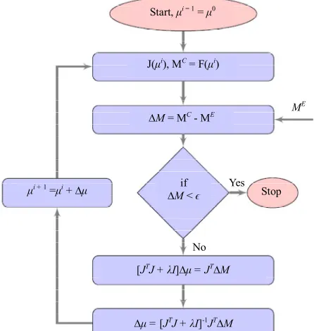
, and J is th e Jacobian matrix which has beenevaluated at each iteration of MoBIIR algorithm (Figure
1). The above equation is the parameter update
expres-sion. In Equation 5, I is the identity matrix whose
dimen-sion is equal to the dimendimen-sion of JTJ. is
regulariza-tion parameter and the order of magnitu of de I should
be near to that of JTJ. The impact of noise a nd on
the reconstruction i discussed in results section The
Figure 1 gives a flow chart of the approach based on Gauss Newton.
s .
Start, μi = 1 = μ0
Stop
ME
Yes
No J(μi), MC = F(μi)
μi + 1 =μi + ∆μ
∆M = MC- ME
if
∆M < ϵ
[JTJ + λI]∆μ = JT∆M
∆μ = [JTJ + λI]-1JT∆M
2.2. Hessian Based Approach
Figure 1. Flowchart for image reconstruction by Newton method based MoBIIR algorithm.
thm recovers an
ap-’s
The iterative reconstruction algori
proximation to from the set of boundary
measure-ments Me. By directly Taylor expanding Equation 3,
and using a quadratic term involving Hessian, the per-turbation equation can be written as,
i1
i i
f f F i
T
i F i i
(6)
where F is the Hessian corresponding to
. Fo
T
the
meas-urement r d number of detectors, the above equation
can be rewritten as, d T
1
.
i i
i
F F F M F
M
(7)The Equation 7 is the update equation obt the
ained from
quadratic perturbation equation. The term F M is
often observed to be diagonally dominant and can be
denoted by ii, neglecting the off diagonal terms. Thus,
through the incorporation of the second derivative term, the update equation has a generalized form with a physi-cally consistent regularization term.
2.3. Broyden Approaches
The major constraint of Newton’s method is the compu-tationally expensive Jacobian evaluation [17,18]. The quasi-Newton methods provide an approximate Jacobian
[19]. Samir et al [5] has developed an algorithm making
use of Broyden’s method [17,18,20] to improve the Jacobian update operation, which happens to be the ma-jor computational bottleneck of Newton-based MoBIIR. Broyden’s method approximates the Newton direction by using an approximation of the Jacobian which is updated as iteration progresses. Broyden method uses the current
estimate of the Jacobian Ji1 and improves it by taking
the solution of the secant equation that is a minimal
modification to Ji1. For this purpose one may apply
rank-one updates. We have assumed that we have a
non-singular matrix J
i and we wish to produce anap-proximate J
i1 through rank-1 updates [21]. Theforward solution be expressed in terms of derivatives
of the forward solution using Taylor expansion as, can
i i1 i1 i i 1 .F F J
(8)
The Broyden’s Jacobian update equation becomes
1
[ ]
i i iT
i
M J Ji Ji i i
1 where .
i i
i
i i i i i i
M J
J J J J
iT
[image:3.595.62.285.469.704.2]Equation 9 is referred to as Broyden’s update equation. In Broyden’s method there is no clue about the in Jacobian estimate [22]. The initial value of Jacobian
itial
0J is computed through analytical methods based
on adjoint principles. It is found that since Jacobian up-date is only approximate, the number of iterations
re-qui Broyden method for convergence is higher
than that of gauss-Newton methods. This can be im-proved by re-calculating Jacobian using adjoint method when Jacobian is found to be outside the confidence do-main (when MSE of the current estimate is less than
MSE of the previous estimate). If the initial guess 0
red by
is
sufficiently close to the actual optical parameter *
then the J
0 is sufficiently close to A
0 and thesolution converges q-superlinearly to *. The most
no-table feature of Broyden approach is that it avoids dire
computati Jacobian, thereby providin ter
algo-rithm for DOT reconstruction.
2.4. Adjoint Broyden Based MoBIIR
Least change secant based Adj
ct
on of g a fas
oint Broyden [23] update method is another approach for updating the system Jacobian approximately.
The direct and adjoint tangent conditions are
11
i i i
i
J F and 1
1T T i
i Ji i F
respectively. With respect to the Frobenius norm .Frob,
the least change update of a matrix Ji to a matrix Ji1
satisfies the direct secant conditi on 1
i i
i
J M and
the adjoint secant condition 1
T T
i Ji i
, for norm d
directions i and alize
i
, and is given s [23] a
1
i i
i iT iT
i
J J r T i iT
i i r
(10)
where i i i
i
r M J
, i T
i Ji i
. The rank-1
update for Jacobian update based on adjoint method is
given as [5],
11 .
T i i i
i i T i
i i
J J F J
(11)
The Adjoint Broyden update is categorized based on
the choice of i. For simplicity, we conside
direction [23] ch is defined as,
r only secant whi
11
with .
i i i
i i i
i i i
i
F F J
(12)
where i
met
is the step size and is estimated through line
search hod. The above equation has bee
Adjoint Broyden based MoBIIR image reconstruction. im
n solved in
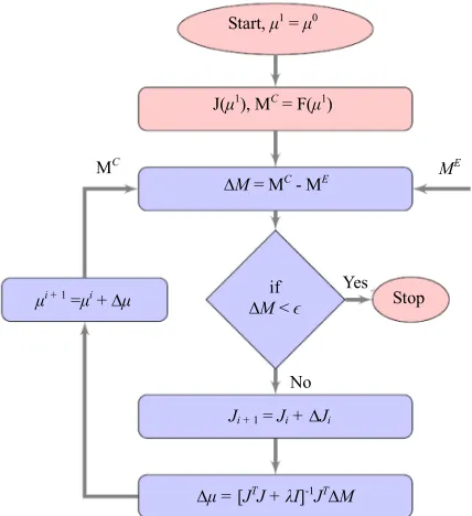
The age reconstruction flowchart using Broyden
based MoBIIR is shown in Figure 2. The Jacobian is
updated through Equation 9 and Equation 11 for Broyden method and adjoint Broyden method respectively.
Start, μ1 = μ0
J(μ1), MC = F(μ1)
Stop ME C
M
C E
∆M = M - M
if
∆M < ϵ μi + 1 =μi + ∆μ
No
Ji + 1 = Ji + ∆Ji
∆μ = [JTJ + λI]-1JT∆M
[image:4.595.317.531.85.319.2]Yes
Figure 2. Flowchart for image reconstruction by Broyden- based MoBIIR (Equation 9) algorithm.
2.5. Pseudo-Dynamic Approaches
used in image re-n. Several in the literature Diffuse optical tomographic imaging is an ill-posed problem, and a regularization term is
construction to overcome this limitatio larization schemes have been proposed
[24]. However, choosing the right regularization pa-rameter is a tedious task. A some what regularization- insensitive route to computing the parameter updates using the normal equations Equation 5 or Equation 7 is to introduce an artificial time variable [25,26]. Such pseudo- dynamical systems, typically in the form of ordinary dif-ferential equations (ODE-s), may then be integrated and the updated parameter vector recovered once either a pseudo steady-state is reached or a suitable stopping rule is applied to the evolving parameter profile (the latter being necessary if the measured data are few and noisy).
Samir et al [5] have used the above approach to arrive at
a DOT image reconstruction.
For the DOT problem, the pseudo-time linearized ODE-s for the Gauss-Newton’s normal equation for
i,i
t t t t is given by:
i,
0s
S t V
i
(13)
d :
dt
, i:
it
, where
i : T
i E
is
V F M F
, and
i,
i iwhen we use Equation 5. For the case where the
quad-ratic perturbation is used (Equation 7), then S is replaced is the stopping time) with ˆ
N
.
by
3. Results
i,
T T TG F F F FI (14)
g the pseudo-time recursion for
Figure 3 gives the reconstruction results with a single
embedded inhomogeneity. Figure 3(a) is the phantom
with one inhomogeneity. The reconstructed images using Newton-based MoBIIR, Broyden-based MoBIIR and adjoint Broyden-based MoBIIR are given in (b), (c), and (d) respectively.
We first consider the linear case wherein Equation 5 is used to arrive at the pseudo-dynamic system. While
initi-atin t
t ti,i t
, theinitial parameter vector 0 may be
to the background value which is assum Eq
taken corr ed to
esponding be known.
Figure 4 gives the performance of the algorithm. It is seen that adjoint Broyden converges faster compared to
other algorithms. Figure 4(a) shows that Newton,
Broy-den and adjoint BroyBroy-den methods converge at ,
and 20 iterations respectively. The cross section
through the center of the inhomogeneities is shown in
Figure 4(b).
16th
22th th
uation 13 may be integrated in closed-form leading to the following pseudo-time evolution,
1
1
1
exp ,
exp , d
i
i
i i i
i
t i
i t
S h
S t t f t t
(15)where
i,
i
is
f t S V and i. In
the ideal data is he
sequence it poi
1
i i
h t t
noise-free, t nt ˆ case, when the measured
; 1, 2, ,
i i N
has a lim
Figure 5 gives the reconstruction results with two
embedded inhomogeneities. Figure 5(a) is the phantom.
The reconstructed images using Newton-based MoBIIR, Broyden-based MoBIIR and adjoint Broyden-based Mo-BIIR are given in (b), (c), and (d).
, which rio
yields the a pr
where i.e,
desired reconstruction. In the measured data is noisy,
actical scena
E E
M M
with being a measure of the no
; 1, 2, ,
i i N
ise ‘str this
case, a stopping rule may have to be imposed so that the
sequence
is stopped at *ength’. In
N t t (t*
Figure 6 gives the performance of the algorithm with two inhomogeneities. MSE of reconstructed images with
two inhomogeneities is shown in Figure 6(a). Figure 6(b)
40
0.018 20
0
-20
-40
-40 -20 0 20 40
40
20
0
-20
-40
-40 -20 0 20 40
0.02
0.016
0.014
0.012
0.01 6.7 mm 11.5 mm
0.01 0.011 0.012 0.013 0.014 0.015
(a) (b)
40
20
0
-20
-40
-40 -20 0 20 40
40
20
0
-20
-40
-40 -20 0 20 40
0.01 0.011 0.012 0.013 0.014 0.015
0.01 0.011 0.012 0.013 0.014 0.015
(c) (d)
Figure 3. (a) Phantom with one inhomogeneity having 0.01 1
a
μ mm and 1 1
s μ mm
BIIR; (d) Adjoint Broy
-45 0
0.01 0.012 -40
-35 -30
5
Iteration 20
0.014 0.016 0.018 0.02
25
Line through the inhomogeneity Newton MoBllR
Broyden MoBllR Adjoint Broyden MoBllR
Newton MoBllR Broyden MoBllR Adjoint Broyden MoBllR Actual Inhomogeneity
Lo
g (
M
S
E)
A
bsorpt
ion C
oef
fi
cient
15 -40 -20 0 20 40
10
(a) (b)
Figure 4. (a) Newton, Broyden and adjoint Broyden methods. They converge at and iterations respectively; (b) Cross-section through the center of inhomogeneities for Newton, Broyden oyde thods.
16th and adjoint Br
, 22th 20th n me
40
20 0.
0.018 0.014
0.015
20
0
-20
-40
-40 -20
40
0
-20
-40
-40 -20 0 20 40
02
0.016
0.014
0.012
0.01 6.7 mm 11.5 mm
0.01 0.011 0.012 0.013
(
0 20 40
a) (b)
40 40
0.016 0.014
20
0
-20
-40
-40 -20 0 20 40
20
0
-20
-40
-40 -20 0 20 40
0.01 0.012 0.014
0.01 0.011 0.012 0.013 0.014 0.015
(c) (d)
Figure 5. (a) Original simulated phantom with two inhomogeneities; The a of the inhomogeneities are 0.02 and 0.015
and are at (0, −192.2) and ewton; (c) Broyden; (d) adjoint
n method.
shows that Newton, Broyden and adjoint Broyden
meth-ods converge at and iterations
respec-tively. The line plot t r of the
[image:6.595.117.481.84.195.2]inhomoge-neities is shown in Figure 6(c).
Figure 7 gives the reconstruction results with two
em-bedded inhomogeneities. Figure 7(a) is the reconstructed
image by Gauss-Newton method. Figures 7(b) and (c)
are the reconstructed images by linear pseudo-dynamic time marching algorithm and by non-linear (Hessian in-tegrated) pseudo-dynamic time marching algorithm re-spectively.
center of inhomogeneities is shown in Figure 8(a). The
variation of the Normalized Mean Square Error (MSE)
with Iteration is shown in Figure 8(b). The blue line
represents Gauss-Newton’s method and green line repre-sents pseudo dynamic time matching algorithm.
4. Conclusion
In this study, we look at many approaches used for solv-ing the DOT problem. Like any medical image main focus is to reconstruct a tio
1
mm
Broyde
(0, 19.2) respectively Reconstructed results using; (b) N
18th, h
37th rough
24th
the cente
[image:6.595.115.480.238.532.2]-45 0 -40 -35
10
Iteration 20 Newton MoBllR Broyden MoBllR Adjoint Broyden MoBllR
L
og
(M
SE
)
-30
30 40
-45 0 -40 -35
10
Iteration 20
Newton MoBllR Broyden MoBllR Adjoint Broyden MoBllR
L
og
(M
SE
)
-30
30 40
A
bso
rp
tion
Co
eff
ic
ient
0.01 0.012 0.014 0.016 0.018 0.02
0 20 40 -40 -20
Line through inhomodeneity
Newton MoBllR Broyden MoBllR Adjoint Broyden MoBllR Actual Target
)
T
im
e (se
c
b) (c)
oge ) Lin it
(a) (
Figure 6. (a) MSE of reconstructed images with two inhom converge at 18th, 37th and 24th iterations respectively; (c ton’s and propo
neities; (b) Newton, Broyden and adjoint Broyden methods e plot through the center of the inhomogeneities using New-sed algor hms.
0 20 40 -40 -20
-20 0 20
0.01 0.015 0.02 0.025
-40 -20 0 20 40
-20 0 20
0.01 0.015 0.02 0.025 40
-40
-40 -20 0 20 40
-20 0 20
0.01 0.015 0.02 0.025
(a) (b) (c)
Figure 7. (a) Reconstructed image by Gauss-Newton method; (b) Reconstructed image by Linear pseudo-dynamic time marching algorithm; (c) Reconstructed image by non-linear (Hessian integrated) pseudo-dynamic time marching algorithm
A
bsor
pt
io
n C
oef
fi
cie
nt
0.01 0.02
0 20 40
-40 -20
Cross-sectional line through the inhomodeneity
Reference
0.03
0.015 0.025
PD Quadratic PD Linear GN
ǁ
M
e -
M
c ǁ
2
0.2
0 20 40
GN
0.8 PD Linear
PD Quadratic
0.6
0.4
0
Recursions/Iterations
10 30
1
problem is non-linear and ill-posed, the iterative methods are often used for solving this type of problems. We have summarized a few studies we undertook towards this. They are 1) Gauss-Newton based MoBIIR; 2) Quadratic Gauss-Newton, Broyden-based MoBIIR; 3) Adjoint Broy- den based MoBIIR, and pseudo-dynamic approaches.
REFERENCES
[1] S. R. Arridge, “Optical Tomography in Medical
Imag-ing,” Inverse Problems, Vol. 15, No. 2, 1999, pp. R41- R93.
[2] S. R. Arridge, M. Schweiger, M. Hiraoka and D. T. Delpy, “Finite Element Approach for Modelling Photon Trans- port in Tissue,” Medical Physics, Vol. 20,1993, pp.299- 309.http://dx.doi.org/10.1118/1.597069
(a) (b)
Figure 8. (a) The cross-sectional line plot through reconstructed inhomogeneity; (b) The variation of the Normalized Mean Square Error (MSE) with Iteration. The blue line represents Gauss-Newton’s method and green line represents pseudo
dy-amic time matching algorithm. n
[image:7.595.72.526.84.209.2] [image:7.595.63.534.263.386.2] [image:7.595.78.517.429.566.2]http://dx.doi.org/10.1088/0031-9155/52/5/013
[4] B. W. Pogue, S. C. Davis, X. Song, B. A. Brooksby, H. Dehghani and K. D. Paulsen, “Image Analysis Methods for Diffuse Optical Tomography,” Journal of Biomedical Optics, Vol. 11, 2006, Article ID: 1033001.
http://dx.doi.org/10.1117/1.2209908
[5] S. K. Biswas, K. Rajan, R. M. Vasu and D. Roy, “Accel-erated Gradient Based Diffuse Optical Tomographic Im-age Reconstruction,” Medical Physics, Vol. 38,2011, p. 539.http://dx.doi.org/10.1118/1.3531572
[6] S. K. Biswas, K. Rajan and R. M. Vasu, “Practical Fully 3-D Reconstruction
mography,” Journal oAlgorithm for Diffuse Optical To-f the Optical Society of America A, Vol. 29, 2012, p. 1017.
http://dx.doi.org/10.1364/JOSAA.29.001017
[7] D. A. Boas, J. P. Culver, J. J. Stott and A. K. Dunn, “Three Dimensional Monte Carlo Code for Photon Mi-gration through Complex Heterogeneous Media Including the Adult Human Head,” Optics Express, Vol.10, No. 3, 2002, pp. 159-170.
http://dx.doi.org/10.1364/OE.10.000159
[8] G. S. Abdoulaev and A. H. Hielscher, “Three-Dimen- sional Optical Tomography with the Equation of Radia- tive Transfer,” Journal of Electronic Imaging, Vol. 12, No. 4, 2003, pp. 594-601.
http://dx.doi.org/10.1117/1.1587730
[9] M. Schweiger, S. R. Arridge and I. Nissila, “Gauss-Newton Method for Image Reconstruction in Diffuse Op- tical Tomography,” Physics in Medicine and Biology, Vol. 50, No. 10, 2005, pp. 2365-2386.
http://dx.doi.org/10.1088/0031-9155/50/10/013
[10] C. K. Hayakawa and J. Spanier, F. Bevilacqua, A. K. Dunn, J. S. You, B. J. Tromberg and V. Venugopalan “Perturbation Monte Carlo Methods to Solve Inv
rlo -Sca
edia,” . 2095-2097.
erse
Photon Migration Problems in Heterogeneous Tissues,”
Optics Letters, Vol. 26, No. 17, 2001, pp. 1335-1337. [11] P. K. Yalavarthy, K. Karlekar, H. S. Patel, R. M. Vasu, M.
Pramanik, P. C. Mathias, B. Jain and P. K. Gupta, “Ex- perimental Investigation of Perturbation Monte-Ca Based Derivative Estimation for Imaging Low ttering Tissue,” Optics Express, Vol. 13, No. 3, 2005, pp. 985- 988.
[12] A. Sassaroli, “Fast Perturbation Monte Carlo Method for Photon Migration in Heterogeneous Turbid M
tics Letters, Vol. 36, No. 11, 2011, pp
Op-
http://dx.doi.org/10.1364/OL.36.002095
[13] B. W. Pogue, M. S. Patterson, H. Jiang and K. D. Paulsen, “Initial Assessment of a Simple System for Frequency Domain Diffuse Optical Tomography,” Physics in Medi- cine and Biology,Vol. 40, 1995, pp. 1709-1729.
http://dx.doi.org/10.1088/0031-9155/40/10/011
[14] T. Tarvainen, M. Vauhkonen, V. Kolemainen, S. R. Ar-ridge and J. P. Kaipio, “Coupled Radiative Transfer
Equation and Diffusion Approximation Model for Photon Migration in Turbid Medium with Low-Scattering and Non-Scattering Regions,” Physics in Medicine and Biol- ogy, Vol. 50, 2005, pp. 4913-4930.
http://dx.doi.org/10.1088/0031-9155/50/20/011
[15] K. Levenburg, “A Method for the Solution of Certain Non-Linear Problems in Least-Squares,” Quarterly of Applied Mathematics, Vol. 2,1944, p. 164.
[16] D. W. Marquardt, “An Algorithm for the Least-Square Estimation of Non-Linear Parameters,” SIAM Journal on Applied Mathematics, Vol. 11, 1963, p. 431.
http://dx.doi.org/10.1137/0111030
ery of the Good Broyden
[18] C. G. Broyden, “A Class of Methods for Solving Nonlin-
omputa-
hnabel, “A
Journal,
Paulsen, “Spatially variant regularization improves [17] C. G. Broyden, “On the Discov
Method,” Mathematical Programming, Vol. 87, No. 2, 2000, p. 209.
ear Simultaneous Equations,” Mathematics of C tion, Vol. 19, 1965, pp. 577-593.
[19] H. Wang and R. P. Tewakson, “Quasi-Gauss-Newton Method for Solving Non-Linear Algebraic Equations,”
Computers & Mathematics with Applications, Vol. 25, 1993, pp. 53-63.
[20] R. H. Byrd, H. Khalfan and R. B. Sc
cal and Experimental Study of the Symmetric Rank One Update,” Technical Report CU-CS-489-90, University of Colorado, 2002
[21] J. Branes, “An Algorithm for Solving Nonlinear Equa-tions Based on the Secant Method,” Computer
Vol. 8, No. 1, 1965, pp. 66-72.
[22] J. E. Dennis Jr. and R. B. Schnabel, “Numerical Methods for Unconstrained Optimization and Nonlinear Equa-tions,” Prentice-Hall, Englewood Cliffs, 1983.
[23] S. Schlenkrich, A. Griewank and A. Walther, “On the Local Convergence of Adjoint Broyden Methods,” Ma- thematical Programming, Vol. 121, No. 2, 2010, pp. 221- 247.
[24] B. W. Pogue, T. McBride, J. Prewitt, U. L. Osterberg and K. D.
diffuse optical tomography,” Applied Optics, Vol. 38, 1999, pp. 2950-2961.
http://dx.doi.org/10.1364/AO.38.002950
[25] B. Banerjee and D. Roy and R. M. Vasu, “A Pseudo-
Pseudo- y under Dynamical Systems Approach to a Class of Inverse Prob-lems in Engineering,” Proceedings of the Royal Society A, Vol. A465, 2009, pp. 1561-1579.
[26] B. Banerjee and D. Roy and R. M. Vasu, “A Dynamic Sub-Optimal Filter for Elastograph
Static Loading and Measurement,” Physics in Medicine and Biology, Vol. 54, 2009, pp. 285-305.