R E S E A R C H
Open Access
Improved BM3D image denoising using
SSIM-optimized Wiener filter
Mahmud Hasan and Mahmoud R. El-Sakka
*Abstract
Image denoising is considered a salient pre-processing step in sophisticated imaging applications. Over the decades, numerous studies have been conducted in denoising. Recently proposedBlock matching and 3D (BM3D) filtering added a new dimension to the study of denoising. BM3D is the current state-of-the-art of denoising and is capable of achieving better denoising as compared to any other existing method. However, there is room to improve BM3D to achieve high-quality denoising. In this study, to improve BM3D, we first attempted to improve the Wiener filter (the core of BM3D) by maximizing the structural similarity (SSIM) between the true and the estimated image, instead of minimizing the mean square error (MSE) between them. Moreover, for theDC-only BM3Dprofile, we introduced a 3D zigzag thresholding. Experimental results demonstrate that regardless of the type of the image, our proposed method achieves better denoising performance than that of BM3D.
Keywords: Image denoising, Image restoration, BM3D, Wiener filter, Structural similarity, Collaborative filtering, Hard thresholding, Mean square error
1 Introduction
There are different types of noise that can contaminate a digital image. Depending on the noise type, there are various algorithms present in the literature for denois-ing the image.Block matching and 3D (BM3D) filtering
[5] is one such popular algorithm that reduces additive white Gaussian noise (AWGN) [16] from digital images. In terms of denoising performance, BM3D is considered the best denoising filter to date. It exhibits remarkable results when compared to other existing methods. BM3D works in two identical steps. In the first step, it generates a basic estimate of the noisy image using hard thresholding. Then in the second step, it uses Wiener filter to actually denoise the noisy image. To do so, BM3D uses the basic estimate generated from the first step as an oracle (i.e., a pilot signal) in the Wiener filter.
Wiener filter is an age-old benchmark for image denois-ing and restoration [23]. This filter needs a degradation function for denoising or restoration. The better the degradation function is, the more denoising is achievable by Wiener filter. BM3D uses the basic estimated image from the first step as the degradation function of Wiener
*Correspondence:[email protected]
Department of Computer Science, Western University, London, Ontario, Canada
filter. Thus, the ultimate performance of BM3D largely depends on how good the basic estimate is.
Although BM3D achieves good denoising performance, it is not sufficient to denoise images contaminated by huge levels of noise. In other words, the performance of BM3D decreases with the increase of noise level. Again, among the different profiles of BM3D (a profile is a specific set of parameters), theDC-onlyprofile (meaning that the 3D transform used is the 3D-DCT) generally performs poorer than the others. Therefore, there is scope to either propose better denoising technique than BM3D or to make BM3D perform better than what it can currently do.
The Wiener filter [23] was proposed about half a century ago. Different researchers attempted to improve the per-formance of the Wiener filter; however, most studies did not directly address one persisting problem of the Wiener filter which is it uses an objective function, called mean square error (MSE), which is often a misleading measure. In other words, it is possible to use a better measure than MSE as the objective function of Wiener filter. Also, if the Wiener filter can be improved, the performance of BM3D can also be improved, since it uses the Wiener filter as one of its fundamental components.
In this study, we will primarily focus on the improve-ment of Wiener filter. Then, we will use this improved
Wiener filter in BM3D to improve its response as well. Our objective is to eventually improve the denoising per-formance of all profiles of BM3D through improving the Wiener filter. Note that the authors previously published their preliminary idea of how the Wiener filter can be improved [9]. In this article, the authors will utilize their previous Wiener improvement idea to further improve the BM3D filtering scheme. In addition, we will also design some additional components to improve the performance of BM3D, especially the performance of BM3D profile. It is worth mentioning that from now on till the end of the article, we will refer toAdditive White Gaussian Noise (AWGN)whenever the termnoiseis used.
The rest of the article is organized as follows. In Section 2, we will discuss the working procedure and parameterized setup of BM3D in details. In Section3, we will discuss the Wiener filter and its variants. In Section4, we will address the existing problems of the Wiener filter and BM3D that we are interested to solve in this study. We will propose our methodologies in Section5 and report their performance in Section6. Finally, we will conclude in Section7discussing some possible future work.
2 Block matching and 3D (BM3D) filtering
In recent years, probably the most discussed denoising technique is block matching and 3D (BM3D) filtering [5]. It was first suggested by Dabov et al. in 2007. Later, it was rigorously reviewed by Lebrun [12]. The idea has become extensively popular in denoising over the last few years. BM3D achieves excellent performance for reducing AWGN noise. In this section, we will discuss BM3D and its different profiles.
2.1 Algorithm of BM3D
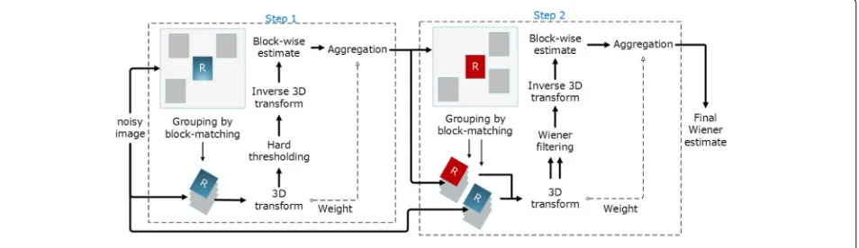
The BM3D algorithm can be simply described in a step by step fashion. Let us start with Fig.1that shows the block diagram of BM3D [5].
BM3D takes the concept of non-local means (NLM) published in 2005 [2] in the sense that it also attempts denoising based on finding similar patches within a given
window. BM3D has two identical steps namely step 1 and step 2. They are identical in the sense that they have no operational difference, rather the difference lies in the component that are used during the two steps. For exam-ple, the first step uses hard thresholding while the second step uses Wiener filtering. Other than that, both steps are identical. BM3D basically tries to denoise the noisy image in the first step to generate a basic estimate. This basic estimate is used in Wiener filtering of the second step as an oracle (i.e., degradation model) [5].
2.1.1 BM3D first step
In step 1, BM3D starts its operation by dividing the noisy image into a number of blocks or patches. For each patch, it then generates a window centering the block being pro-cessed. BM3D defines this center patch as a reference patch. Then, within this window, BM3D looks for the patches similar to the reference patch. Usually, a good number of similar patches are found. BM3D defines a threshold that decides whether two patches are similar or not (see Table1). Once the similar patches are found, BM3D stacks all the similar patches together thus building a 3D block, where the first patch is the reference patch and others patches are sorted according to their distance to the reference patch. BM3D allows a number of 3D trans-form techniques to transtrans-form the domain from spatial to frequency (as indicated by the 3D transform in Fig. 1). After the 3D transform is performed, the most impor-tant part of the first step, known as hard thresholding, is executed. Hard thresholding is a filter that allows any coefficient with absolute value above a certain threshold to pass through, while converts the remaining coefficients to zero. This is the only operation in the first step that per-forms denoising, the rest are only to make a platform for hard thresholding. After hard thresholding, BM3D tries to generate a basic estimate. For this, it needs to trans-form the block coefficients to intensity values in the spatial domain. This is known as inverse 3D transform. After performing the inverse 3D transform, what is obtained is the 3D block that we started working with. But this time,
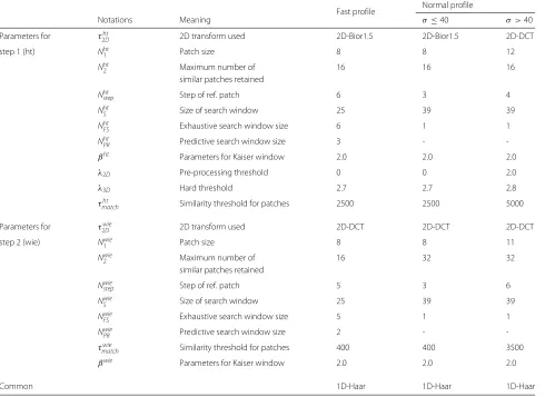
Table 1Parameterized setup for the wavelet profile of BM3D
Fast profile Normal profile
Notations Meaning σ≤40 σ >40
Parameters for τht
2D 2D transform used 2D-Bior1.5 2D-Bior1.5 2D-DCT
step 1 (ht) Nht
1 Patch size 8 8 12
Nht
2 Maximum number of 16 16 16
similar patches retained
Nhtstep Step of ref. patch 6 3 4
Nht
S Size of search window 25 39 39
Nht
FS Exhaustive search window size 6 1 1
Nht
PR Predictive search window size 3 -
-βht Parameters for Kaiser window 2.0 2.0 2.0
λ2D Pre-processing threshold 0 0 2.0
λ3D Hard threshold 2.7 2.7 2.8
τht
match Similarity threshold for patches 2500 2500 5000
Parameters for τwie
2D 2D transform used 2D-DCT 2D-DCT 2D-DCT
step 2 (wie) Nwie
1 Patch size 8 8 11
Nwie
2 Maximum number of 16 32 32
similar patches retained
Nwiestep Step of ref. patch 5 3 6
NwieS Size of search window 25 39 39
Nwie
FS Exhaustive search window size 5 1 1
Nwie
PR Predictive search window size 2 -
-τwie
match Similarity threshold for patches 400 400 3500
βwie Parameters for Kaiser window 2.0 2.0 2.0
Common 1D-Haar 1D-Haar 1D-Haar
it is denoised. Now, for each patch in the 3D block, an aggregation to estimate the reference patch is made. This aggregation is simply taking different weights and estimat-ing each pixel. Once the aggregation is done, the basic estimate is ready to start the second step.
In theory, it is obvious that the more patches are present in the 3D block, the better estimates will be found for one single pixel as well as the better denoised basic estimates. However, according to Dabov et al. [5], in practice, it is seen that after a certain number of similar patches, BM3D does not seem to perform better.
2.1.2 BM3D second step
The second step is similar to the first step with two small differences. First, the 3D grouping is now performed on a basic estimate that was obtained from the first step, not on the noisy image as in step 1. Second, the hard threshold-ing is not used any more after the 3D transform. Instead, a Wiener filter is now used. We will discuss in Section3 that the Wiener filter needs a degradation functionH()to work. In BM3D, the 3D group built on the basic estimate
is considered as the degradation function for BM3D while the corresponding 3D group of the noisy image is the degraded image functionG().
Equation 1 shows how the Wiener filter works in BM3D. Here,Pbasic(P)(ξ)is the 3D block from the basic image andP(P)is the corresponding 3D block from the noisy image.τ3wienD denotes the 3D transformation for the Wiener filter phase. Once the inverse 3D transform of Eq. 1 is computed,Pwien(P) is found which is the final estimate for one block. Once the estimate is obtained, a weighted aggregation operation, like in step 1, is per-formed to build the final denoised image.
ωp(ξ)=
τwien
3D Pbasic(P)(ξ) 2
τwien
3D Pbasic(P)(ξ) 2
+σ2 ·τ wien
3D P(P) (1)
2.1.3 Parameters and profiles of BM3D
wavelet profile. In DC-Only profile, BM3D uses a three-dimensional discrete cosine transform as a 3D transform. For the wavelet profile, on the other hand, BM3D uses a combination of 2D bi-orthogonal transform and 1D-Haar or Walsh-Hadamard transform. DC-only profile gener-ally produces poorer results as compared to its wavelet counterpart [5, 6]. Wavelet profile may be defined as the mainstream BM3D since the authors of BM3D [5] recommended to use Wavelet transform in their pro-posed denoising method. This is because, the main stream BM3D has PSNR gain much better than DC-only profile. For the wavelet profile, we used an exactly same parame-terized setup as in BM3D [5]. We present the basic param-eterized setup from the original article [5] in Table1for readers’ convenience. We use exactly the same parameters to ensure the same environment for the experiment. The wavelet profile uses two sub-profiles called normal pro-fileandfast profile. The only difference between them is that the denoising performance is compromised in order to reduce the computational complexity in fast profile. Another difference between these two profiles is thefast profileuses predictive searching in order to decrease its searching time while thenormal profileuses only exhaus-tive searching.
3 Wiener filter revisited
A Wiener filter provides an opportunity to deal with both noises and degradation. This feature makes the Wiener fil-ter unique in both image denoising and restoration. This filter is also called minimum mean square error. This is because the core idea behind the Wiener filter is to sat-isfy an objective function which is the mean square error (MSE). In other words, this guarantees that the image restored by the Wiener filterfˆ will have minimum MSE with respect to original uncorrupted imagef. Equation2 shows that the expectation of a Wiener filter is to have minimum MSE betweenf andˆf.
e2=E(f − ˆf)2 (2)
The Wiener filter is defined by Eq.3. Note that all terms are given in the transformed domain. Here,H(u,v)is the degradation function, H∗(u,v) is the conjugate complex ofH(u,v),Sn is the power spectrum of noise defined as Sn = |N(u,v)|2, andSf is the power spectrum of
unde-graded image defined as Sf = |F(u,v)|2. G(u,v) is the
transform of the degraded image, andFˆ(u,v)is the final estimate for the restored image. Once the inverse trans-form of Fˆ(u,v)is computed,fˆ(x,y)is obtained which is the denoised/restored approximation for original image
f(x,y).
ˆ
F(u,v)= H
∗(u,v)
|H(u,v)|2+Sn Sf
G(u,v) (3)
Comparing Eq. 1 with Eq. 3, it is evident that both equations are exactly the same, except that Eq.1 works with 3D data. Equation3can be solved forG(u,v) as in Eq.4and rewrite Eq.4as in Eq.5.
G(u,v)= H
∗(u,v)S
f(u,v)) |H(u,v)|2Sf(u,v)+Sn(u,v)
(4)
G(u,v)= 1 H(u,v)
⎡
⎣ |H(u,v)|2
|H(u,v)|2+Sn(u,v) Sf(u,v)
⎤
⎦ (5)
Now, if the noise is zero, the term inside the square brackets in Eq. 5 becomes 1, which means the Wiener filter is reduced to an inverse filter and works for only restoration. However, if there is noise, the Wiener fil-ter incorporates itself for removal of noise along with restoration. This is what makes the Wiener filter unique.
4 Existing problems with Wiener filter and BM3D 4.1 Wiener filter objective function
4.1.1 MSE-optimized Wiener filter
As stated in Section 3, a Wiener filter tries to mini-mize its objective function shown in Eq.2while denois-ing/restoring a degraded image. This function is also known as mean square error (MSE) as defined in Eq.6.
MSE= 1
m×n m−1
i=0 n−1
j=0
[I(i,j)− ˆI(i,j)]2 (6)
In this Equation, I and ˆI are considered as the true (or noise free) image and the reconstructed (or denoised) image, respectively. As the difference between these two gets smaller the closer the images are. Also, increased closeness indicates a more accurately denoised image. With this fundamental property, MSE is being used as an image quality metric [13].
The Wiener filter (Eq. 3) guarantees that the denoised/restored image is the closest image possible to the true undegraded image, since this filter is optimized for MSE. We might conclude at this point that in the best-case scenario the Wiener filter may reconstruct an image whose MSE with respect to the true image is zero. That is, both images are exactly the same. However, there are still problems with the typical use of MSE that prevent the Wiener filter from achieving more accurate and perfect results.
4.1.2 Structural similarity
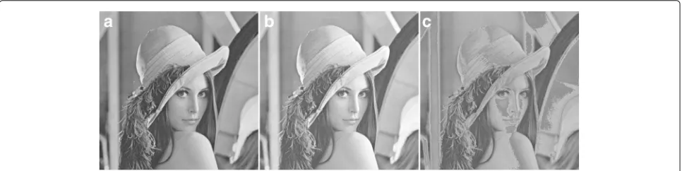
of point-to-point distance measurement. Figure2shows such an example of misleading of MSE measure. In this figure, we used the well-known Lena image in Fig.2aand added a constant 30 to all of its pixel values in order to increase its brightness. The brightened image is shown in Fig.2b. Although there is no visual distortion in the image, the calculated MSE between them is 900. This value is not negligible, and hence MSE cannot be considered as a true error measure.
Now, let us also consider Fig.2c. This is similar to Fig.2b except that now we have not just added a positive constant to all brightness levels, instead, if the brightness value is less than 150, we subtracted 30 from it; otherwise, we added 30. Due to the presence of the square term in Eq.6, the MSE still generates the same error value (900) as in Fig.2, even though the image in Fig.2cis greatly distorted, if it is compared with the image in Fig.2b.
To avoid such misleading error situations, Wang et al. [20] proposed that modern image quality measurement metrics should not depend only on point-to-point dis-tances, it should also consider the geometric or structural similarity between the images. Otherwise, there is a pos-sibility to have the same error results for different images as depicted above. Thus, they proposed a new error mea-surement metric calledstructural similarity (SSIM). Their proposed error measure, SSIM, is defined in Eq.7.
SSIM(x,y)= (2μxμy+c1)(2σxy+c2) μ2
x+μ2y+c1
σ2
x +σy2+c2
(7)
In this Equation,xandydenote two blocks of the same position from the true image and the reconstructed image. μxandμydenote the arithmetic mean or average ofxand yblocks, respectively.σx2andσy2indicate the variance of
xandyblocks, respectively, whileσxyis the co-variance
betweenx and y. c1 and c2 are two constants to
stabi-lize the division with weak denominator and their values are calculated using Eqs.8and9, respectively. Here,Lis the dynamic range of the image whilek1 andk2are two
constants whose values are k1 = 0.01 and k2 = 0.03,
respectively [20,21].
c1=(k1L)2 (8)
c2=(k2L)2 (9)
This measure is calculated block by block. Therefore, a mean SSIM of all blocks is used to represent the final SSIM index value for the whole image. The SSIM index generally varies between−1 to+1 which is often taken as abso-lute to avoid a negativity value. Thus, the SSIM index is a fractional number between 0 and 1 (inclusive), where a 0 indicatesno similarityand a 1 indicatesexact similarity
between two images. Using this measure, we have 0.9650 and 0.7850 for Fig.2b,c, respectively, which indicates that Fig.2cis much more distorted than Fig.2b. This distortion was overlooked by MSE.
There are other misleading measures of MSE; however, we will not cover them in this study. For a detail list of misleading characteristics of MSE, we refer the reader to the literature [10,20–22].
4.2 Existing problems of BM3D
4.2.1 Higher noise levels
BM3D has poor denoising performance to images cor-rupted by higher levels of noise as compared to its response to images corrupted by lower levels of noise. In other words, BM3D’s performance decreases as the noise level increases.
4.2.2 Poor performance of BM3D for DC-only profile BM3D requires the hard thresholding to be performed in a transform domain, after the 3D transform is performed on the similar image blocks. This 3D transform can be either a 2D+1D transform or a 3D transform. In BM3D, usually a 3D Wavelet is used as 3D transform or a combination of 2D-DCT plus a 1D wavelet transform. However, the transform choice is not restricted. If the 3D-DCT is used, this profile is called DC-only profile. Note that, a profile
is basically a set of parameters that is used in BM3D. In the DC-only profile, coefficients are categorized into two categories: DC and AC coefficients, where the DC coeffi-cient preserves the average of the block intensity, which is a significant piece of block information. It is worth men-tioning that the DC coefficient might also possess some noise. When BM3D uses hard thresholding to get rid of the noise in the transform domain, it does not really treat the AC and the DC coefficients differently. As a result of this, the final outcome of DC-only profile is poorer than other profiles (e.g., wavelet profiles).
5 Proposed method
5.1 SSIM-optimized Wiener filter
From the discussion in Section4.1, it is evident that the MSE is not adequate for assessing the closeness between two images, it is rather good at assessing the distance between them. Instead, the SSIM is a more acceptable alternative. This is because, MSE deals with image data while SSIM deals with image information.
It should be noted that the idea of optimizing the Wiener filter with other quality measurement objective functions were tested by a number of objective functions such as sum of absolute difference (SAD) and median of absolute difference (MAD). However, since most of the similarity measures are rather closeness measures based on differences of pixels’ intensities and not on visual similarities, they could not actually further optimize the Wiener filter. Therefore, the choosing of SSIM as an objec-tive function was logical.
The optimization of a denoising filter by SSIM instead of MSE is not very recent. Channappayya et al. in [3, 4] showed that any linear filter can be optimized by SSIM. They compared their proposed SSIM-optimized fil-ter’s result with the MSE-optimized Wiener filter. Their reported results showed that they were able to achieve a higher SSIM value compared to the MSE-optimized Wiener filter; however, their PSNR gain was still poorer than the MSE-optimized Wiener filter.
An SSIM-optimized Wiener filter, which we proposed earlier [9], considers the structural similarity between the reconstructed image and the true image. Since higher SSIM index indicates more similar images, our proposed Wiener filter’s target is to estimate an image which has maximum SSIM possible. In this case, the expectation function of the Wiener filter becomes Eq.10which now needs to be maximized. In Eq. 10, E is the expecta-tion and f andfˆ are the true and reconstructed images, respectively.
e=E{ssim(f,fˆ)} (10)
Having defined the expectation function, our target is to ensure that our designed Wiener filter maximizes our expectation. Taking a careful look at Eq.3, we realize that replacing the term Sn
Sf by a variableK is reasonable and
finding a suitable value of K is possible [7]. Therefore, for our proposed case, we can start with the lowest pos-sible value of K and loop through the highest possible value ofK. For eachK, we record the SSIM error measure
Table 2Performance comparison of normal profile and proposed method
Noise BM3D Proposed PSNR % PSNR BM3D Proposed SSIM % SSIM
level PSNR PSNR gain gain SSIM SSIM gain gain
10 34.17 34.16 – 0.01 – 0.029% 0.903 0.903 0.000 0.000%
20 31.04 31.10 0.06 0.002% 0.843 0.844 0.001 0.119%
30 29.08 29.28 0.20 0.688% 0.789 0.795 0.006 0.760%
40 27.42 27.87 0.45 1.641% 0.731 0.751 0.020 2.736%
50 26.79 27.05 0.26 0.971% 0.702 0.719 0.017 2.422%
60 25.85 26.28 0.43 1.663% 0.656 0.690 0.034 5.183%
70 25.06 25.65 0.59 2.354% 0.615 0.664 0.049 7.967%
80 24.37 25.11 0.74 3.037% 0.575 0.641 0.066 11.478%
90 23.70 24.59 0.89 3.755% 0.534 0.617 0.083 15.543%
100 23.15 24.18 1.03 4.449% 0.500 0.600 0.100 20.000%
in a vector and then restore the image using that K for which the error has been recorded maximum. Thus, for a given range of noise level, it is guaranteed that our pro-posed Wiener filter should be SSIM optimized. Likewise, it should also provide better denoising and restoration.
Since the core of our proposed improvement over BM3D is the SSIM-optimized Wiener filter, interested readers may want to compare the performance given by both SSIM- and MSE-optimized Wiener filter. We refer the reader to our previously published work [9].
5.2 3D zigzag thresholding
In the discrete cosine transform, the first coefficient is basically the average of all pixel values within a given block [17]. Therefore, for a precise inverse transforming result, the accurate DC coefficient is crucial. In order to make sure that the inverse transformation result is the product of vital block information, our proposed method does not apply hard thresholding on the DC coefficient. Instead, it only applies hard thresholding on AC coeffi-cients. The AC coefficients carry various block frequency information [1,7,17]. This information varies from low-frequency to high-low-frequency information. Thresholding all AC coefficients in the same manner might lead to los-ing some significant information, while preservlos-ing some other insignificant information.
In order to keep the most meaningful block information and just reduce the noise, we should use a zigzag thresh-olding, instead of a hard thresholding. Zigzag threshold-ing is realized by applythreshold-ing little or no thresholdthreshold-ing on the DC coefficient and first few AC coefficients and then applying an increasingly higher thresholding on the rest of the AC coefficients (the higher the frequency, the more thresholding is applied). Determining the actual zigzag thresholding value can be chosen using a gamma curve. A gamma curve is as simple asλ3D = κγ, whereκis the
coefficient value,γ is a positive value≥1 that is directly
proportional to the coefficient number, and λ3D is the
thresholded value. Whenγ =1, the relation becomes lin-ear. Using this thresholding scheme, we gradually increase the thresholding effect with the increase of the coefficient number. Note that this3D zigzag thresholding proposal applies to only DC-only profile of BM3D and not to the actual wavelet profile.
6 Results and discussion
6.1 Data set and parameterized setup
We used eight standard gray scale test images for our experiment. The images used are shown in Fig.3.
Table 3Performance comparison of fast profile and the proposed method
Noise BM3D Proposed PSNR % PSNR BM3D Proposed SSIM % SSIM
level PSNR PSNR gain gain SSIM SSIM gain gain
10 34.18 34.17 –0.01 –0.029% 0.904 0.903 –0.001 –0.111%
20 31.04 31.09 0.05 0.161% 0.844 0.844 0.000 0.000%
30 29.07 29.27 0.20 0.688% 0.789 0.795 0.006 0.760%
40 27.45 27.91 0.46 1.676% 0.732 0.752 0.020 2.732%
50 26.81 27.06 0.25 0.932% 0.703 0.720 0.017 2.418%
60 25.89 26.30 0.41 1.583% 0.658 0.690 0.032 4.863%
70 25.07 25.63 0.56 2.234% 0.614 0.663 0.049 7.980%
80 24.38 25.11 0.73 2.994% 0.575 0.641 0.066 11.478%
90 23.76 24.64 0.88 3.704% 0.534 0.621 0.087 16.292%
100 23.14 24.17 1.03 4.451% 0.500 0.600 0.100 20.000%
For all these images, we recorded the responses of a MSE-optimized Wiener filter and our proposed SSIM-optimized Wiener filter. All performance comparison tables reported in this article are based on the average per-formance on these eight test images for each noise level. The noise level is generated using Eq.11where the value ofσ is varied from 0 (minimum) to 100 (maximum) with μ = 0 (zero-mean). Here,σ is known as noise standard deviation. All other parameters are used with their default values as suggested by Dabov et al. [5] and presented in Table1.
p(z)= √1
2πσe
−(x−μ)2
2σ2 (11)
Experimental results presented in this article are reported in both subjective and objective forms. We used peak signal to noise ratio (PSNR) and structural similar-ity (SSIM) as our objective measure. As for the subjec-tive assessment, the output from BM3D and from our proposed method is used to visually comapre the per-formance. While we present the result of all noise level experiments in the objective measure, we only present one noise level in the subjective assessment. We did so in order to keep the number of pages within the allowable limit.
6.2 Performance analysis of wavelet profile
6.2.1 Normal profile
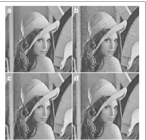
Since the Wavelet profile itself exploits higher perfor-mance as compared to the DC-only profile, even a small increase in PSNR/SSIM indicates a reasonable improve-ment. The experimental results for this profile are given in Table2. The subjective measure is given in Fig.4for Lena image withσ =50.
6.2.2 Fast profile
The fast profile is similar to the normal profile, except that this profile is faster, as the identification of similar blocks is predicted. The performance of the fast profile
is slightly lower than normal profile. The experimental results obtained for fast profile is presented in Table 3. Figure5shows a subjective measure for the Lena image withσ =50.
6.3 Extension of wavelet profile for color image denoising
One approach to employColor BM3D (CBM3D)to 24-bit true color images is to apply BM3D separately on each of its channels. However, correct grouping is one of the key properties of BM3D and it largely depends on the noise level. Again, grouping is a time consuming operation, doing it thrice makes the algorithm considerably slower.
Table 4Performance comparison of color profile (normal) and proposed method
Noise BM3D Proposed PSNR % PSNR BM3D Proposed SSIM % SSIM
level PSNR PSNR gain gain SSIM SSIM gain gain
10 34.11 34.11 0.00 0.000% 0.937 0.937 0.000 0.000%
20 31.29 31.35 0.06 0.192% 0.896 0.897 0.001 0.112%
30 29.56 29.70 0.14 0.474% 0.860 0.864 0.004 0.465%
40 27.92 28.14 0.22 0.788% 0.818 0.824 0.006 0.733%
50 27.61 27.80 0.19 0.688% 0.798 0.806 0.008 1.003%
60 26.81 27.06 0.25 0.932% 0.768 0.781 0.013 1.693%
70 26.07 26.43 0.36 1.381% 0.737 0.757 0.020 2.714%
80 25.47 25.93 0.46 1.806% 0.710 0.737 0.027 3.803%
90 24.89 25.42 0.53 2.129% 0.682 0.717 0.035 5.132%
100 24.23 24.85 0.62 2.558% 0.649 0.692 0.043 6.626%
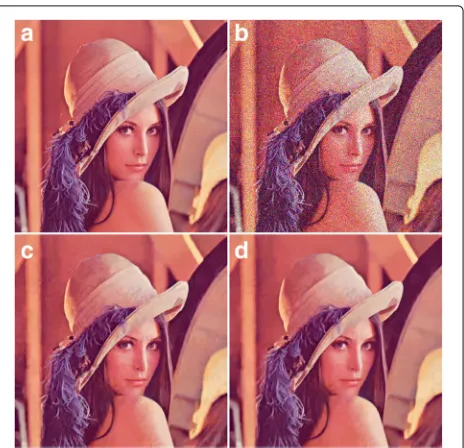
Moreover, three channels should generate three different groupings with sparsity of image information which lead to erroneous hard thresholding. BM3D extension to color image denoising is realized by converting a noisy RGB image into a luminance and chrominance transformed space. In this transformed space, the luminance signal contains most of the image information while the chromi-nance signals contain low-frequency information. There-fore, CBM3D performs grouping on luminance channel only and uses exactly the same grouping for chrominance channels. The idea behind this form of grouping is that if the luminance of two blocks are mutually similar, then the chrominance of these blocks are also mutually similar [5]. We used the same concept for color image denoising as in CBM3D except that in step 2, we used our improved Wiener filter instead of the existing Wiener filter. The experiments are performed for both normal and fast pro-files. The experimental results for normal color profile are presented in Table 4. For visual inspection of denoised color images of normal profile of Lena image withσ =50, we refer the reader to Fig.6.
For the fast color profile, the experimental results are shown in Table5. The output is shown in Fig.7for Lena image withσ = 50 for a visual inspection of the reader. Since the fast profile compromises the performance in order to reduce time, the output is poorer than the normal profile. Therefore, for the image presented forσ = 50 in Fig.7, it may not depict a visible difference; however, this will be evident at higher noise levels.
6.4 Performance analysis of DC-only profile
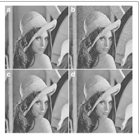
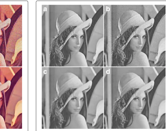
Figure8 shows a comparison between the performance of the proposed zigzag thresholded result and that of BM3D for DC-only profile, where Fig. 8a is the origi-nal image, Fig.8bis the noisy image (σ = 20), and Fig. 8c, dare the output produced by BM3D (DC-only) and the proposed method, respectively. The results show an
improvement in the quality of the denoised image when the proposed method is applied, especially at the face and shoulder areas. For further experimental results on the performance of DC-only profile, readers are referred to Hasan [8].
6.5 Discussion
So far, we have presented a portion of our objective and subjective results from our experimentation. We have also compared our proposed method with the original BM3D. Objectively, our proposed method was able to produce
Fig. 6Subjective assessment between the color normal profile of BM3D and the proposed method.aOriginal image.bNoisy image at noise levelσ =50,PSNR=14.81, andSSIM=0.5495.cOutput using the normal profile of BM3D,PSNR=29.55 andSSIM=0.9741.d
Output using the proposed method,PSNR=29.89 and
Table 5Performance comparison of color profile (fast) and proposed method
Noise BM3D Proposed PSNR % PSNR BM3D Proposed SSIM % SSIM
level PSNR PSNR gain gain SSIM SSIM gain gain
10 33.95 33.96 0.01 0.029% 0.936 0.936 0.000 0.000%
20 31.00 31.09 0.09 0.290% 0.893 0.894 0.001 0.112%
30 29.05 29.28 0.23 0.792% 0.852 0.857 0.005 0.589%
40 27.32 27.59 0.27 0.988% 0.804 0.811 0.007 0.871%
50 27.38 27.54 0.16 0.584% 0.795 0.802 0.007 0.881%
60 26.50 26.77 0.27 1.019% 0.765 0.775 0.010 1.307%
70 25.78 26.12 0.34 1.319% 0.738 0.752 0.014 0.543%
80 25.13 25.57 0.44 1.751% 0.710 0.730 0.020 2.817%
90 24.42 24.96 0.54 2.211% 0.681 0.707 0.026 3.818%
100 23.69 24.22 0.53 2.237% 0.648 0.676 0.028 4.321%
higher PSNR and SSIM values than that of the original BM3D method. Tables 2, 3, 4, and 5 show that as the amount of noise increases, the proposed method man-aged to produce better denoising output, when compared to the original BM3D. For monochrome images, theSSIM gain by the proposed method was as high as 20% while thePSNR gainwas as high as 4.49%. For color images, we achieved slightly less, as the maximum SSIM and PSNR gain were 6.63 and 2.56%, respectively. Subjectively, the quality of the denoising by the proposed method was bet-ter than that by the original BM3D. This was especially
Fig. 7Subjective assessment between the color fast profile of BM3D and the proposed method.aOriginal image.bNoisy image at noise levelσ =50,PSNR=14.81, andSSIM=0.5495.cOutput using the fast profile of BM3D,PSNR=29.29 andSSIM=0.9724.dOutput using the proposed method,PSNR=29.57 andSSIM=0.9740
visible in the flat areas of the images, e.g., Lena’s shoulder and face. It is evident from the results that our pro-posed method achieved better objective and subjective denoising quality.
7 Conclusions
In this study, we rigorously reviewed the current state-of-the-art image denoising scheme (BM3D) as well as its core component, the Wiener filter. We proposed an improved Wiener filter optimized for SSIM that has essentially improved the performance of BM3D. Through
a number of experiments, we proved that our pro-posed Wiener filter, when used in BM3D, is capable of achieving high-quality image denoising. Our idea works for both monochrome (gray scale) and color images. As a brief summary, our novel contributions in this study are the following: (1) reviewing the state-of-the-art image denoising method BM3D with its components and profiles, (2) finding its existing shortcomings, (3) sug-gesting an improved Wiener filter optimized for SSIM [9], (4) using the SSIM-optimized Wiener in BM3D as its core component, and (5) thereby proving that the performance of original BM3D has been significantly improved in our proposed method (through detailed comparative studies via calculating a number of perfor-mance measurement metrics). (6) In addition, we have also proposed a technique named 3D zigzag threshold-ing for improvthreshold-ing the poor performance of DC-only profile of BM3D. All the innovations are discussed in detail in Section 5 while the performed tests, mea-surement metrics, and obtained results are discussed in Section6.
7.1 Future direction
There are other variants of recently proposed SSIM called multi-scale structural similarity (MS-SSIM) [19]. Also, there are other image quality measurement metrics such as image quality index (IQI) [18], Normalized Correlation [11], Sum of Absolute Differences, and many others [15]. A possible future work will test our proposed method by using all of these measures. Recently, BM3D has been extended for video denoising. Also there is BM4D [14]. Since our idea is to change the core ofBMxDin general, a study of assessing our method in allBMxDversions will be considered. In addition, there are recent works such as finding visually similar images using a convolutional deep neural network [24], it would be interesting to study if finding a similarity between images with deep neural net-works helps in forming a quality metric that can eventually be used in a Wiener filter. Also, applying our improved denoising method could help in reducing noise for appli-cations such as text extraction from complex background images [25].
Abbreviations
AWGN: Additive white Gaussian noise; BM3D: Block matching and 3D filtering; BM4D: Block matching and 4D filtering; BMxD: Block matching and xD filtering; CBM3D: Color block matching and 3D filtering; DCT: Discrete cosine transform; IQI: Image quality index; MAD: Median of absolute difference; MS-SSIM: Multi-scale structural similarity; MSE: Mean square error; NLM: Non-local means; PSNR: Peak signal to noise ratio; RGB: Red-green-blue; SAD: Sum of absolute difference; SSIM: Structural similarity
Acknowledgements
Not applicable.
Funding
This research is partially funded by the Natural Sciences and Engineering Research Council of Canada (NSERC). This support is greatly appreciated.
Availability of data and materials
The datasets supporting the conclusions of this article are included within the article.
Authors’ contributions
MES suggested the idea. MH devised the algorithm based on that and carried out the experiments. MES continuously supervised the experiments and suggested modifications. MH prepared the manuscript draft, and MES edited and proof read the manuscript. All authors read and approved the final manuscript.
Competing interests
The authors declare that they have no competing interests.
Publisher’s Note
Springer Nature remains neutral with regard to jurisdictional claims in published maps and institutional affiliations.
Received: 28 August 2016 Accepted: 23 March 2018
References
1. N Ahmed, T Natarajan, K Rao, Discrete cosine transform. IEEE Trans. Comput.C-23(1), 90–93 (1974)
2. A Buades, B Coll, J-M Morel, A non-local algorithm for image denoising. IEEE Conf. Comput. Vis. Pattern Recognit. (CVPR’05).2, 60–65 (2005) 3. S Channappayya, A Bovik, R Heath, A linear estimator optimized for the
structural similarity index and its application to image denoising. Int. Conf. Image Process. (ICIP’06). 2637–2640 (2006)
4. S Channappayya, A Bovik, C Caramanis, R Heath, Design of linear equalizers optimized for the structural similarity index. IEEE Trans. Image Process.17(6), 857–872 (2008)
5. K Dabov, A Foi, V Katkovnik, K Egiazarian, Image denoising by sparse 3-D transform-domain collaborative filtering. IEEE Trans. Image Process.16(8), 2080–2095 (2007)
6. K Dabov, A Foi, V Katkovnik, K Egiazarian, BM3D image denoising with shape-adaptive principal component analysis. Signal Process. Adapt. Sparse Struct. Representations (SPARS’09). (2009)
7. R Gonzalez, R Woods,Digital Image processing, 4th Ed. (Pearson, New York, 2018)
8. M Hasan,BM3D image denoising using SSIM optimized Wiener filter. (Masters Dissertation, Western University, 2014)
9. M Hasan, M El-Sakka, Structural similarity optimized Wiener filter: a way to fight image noise. Int. Conf. Image Anal. Recognit. Lect. Notes Comput. Sci.9164, 60–68 (2015)
10. A Hore, D Ziou, Image quality metrics: PSNR vs. SSIM. Int. Conf. Pattern Recognit. (ICPR’10). 2366–2369 (2010)
11. V Laparra, J Muñoz-Marí, J Malo, Divisive normalization image quality metric revisited. J. Opt. Soc. Am. A.27(4), 852–864 (2010)
12. M Lebrun, An analysis and implementation of the BM3D image denoising method. Image Process On Line.2, 175–213 (2012)
13. E Lehmann, G Casella,Theory of point estimation, 2nd edn. (Springer-Verlag, New York, Berlin Heidelberg, 1998)
14. M Maggioni, V Katkovnik, K Egiazarian, A Foi, Nonlocal transform-domain filter for volumetric data denoising and reconstruction. IEEE Trans. Image Process.22(1), 119–133 (2013)
15. A Mittal, A Moorthy, A Bovik, No-reference image quality assessment in the spatial domain. IEEE Trans. Image Process.21(12), 4695–4708 (2012) 16. Vaseghi S,Advanced digital signal processing and noise reduction, 4th Ed.
(Wiley, Chichester, 2009)
17. G Wallace, The JPEG still picture compression standard. IEEE Trans. Consum. Electron.38(1), xviii–xxxiv (1992)
18. Z Wang, A Bovik, A universal image quality index. IEEE Signal Process. Lett.
9(3), 81–84 (2002)
19. Z Wang, E Simoncelli, A Bovik, Multiscale structural similarity for image quality assessment. Asilomar Conf. Signals, Syst. Comput.2, 1398–1402 (2003)
21. Z Wang, A Bovik,Modern image quality assessment: Synthesis Lectures on Image, Video, and Multimedia Processing. (Morgan and Claypool Publishers, San Rafael, 2006)
22. Z Wang, A Bovik, Mean squared error: love it or leave it? A new look at signal fidelity measures. IEEE Signal Proc. Mag.26(1), 98–117 (2009) 23. N Wiener,Extrapolation, interpolation, and smoothing of stationary time
series. (MIT press Cambridge, Cambridge, 1964)
24. C Yan, H Xie, D Yang, J Yin, Y Zhang, Q Dai, Supervised hash coding with deep neural network for environment perception of intelligent vehicles. IEEE Trans. Intell. Transp. Syst.19(1), 284–95 (2018)
25. C Yan, H Xie, S Liu, J Yin, Y Zhang, Q Dai, Effective Uyghur language text detection in complex background images for traffic prompt