Journal of Chemical and Pharmaceutical Research, 2014, 6(6):1303-1314
Research Article
CODEN(USA) : JCPRC5
ISSN : 0975-7384
Research on recommendation algorithm based on unified model
with explicit and latent factors
Wang Fang
Mechanical and Electronic Engineering Department, Dezhou University, Dezhou Shandong, China
_____________________________________________________________________________________________
ABSTRACT
Recommendation algorithm is one of the major approaches to solve the information overload problem. The core task is to model and predict users’ preference. The algorithms based on the latent factor model have been made a great success recently. However, data sparseness could lead to the incompleteness of the factors in this completely data-driven modeling. To address this issue, this paper leverages certain knowledge of the influencing factors on user preferences to optimize the structure of latent factor model. This paper proposes a unified model with both explicit factors and latent factors. User demographic features and item content features are used as the clues reflecting users’ preferences. These features are introduced to the framework of latent factor model in the form of explicit factors. Experiments on MovieLens dataset suggest that the proposed method is feasible and effective.
Key words: recommendation algorithm; latent factor model; explicit factors
_____________________________________________________________________________________________
INTRODUCTION
With the rapid development of Internet technology, information overload is a problem to be addressed urgently. Information consumers want to be able to get the desired information quickly and efficiently. The producers of information, such as e-commerce sites, are eager to find potential customers to increase profitability and improve the user’s experience. In the context of such a demand, it is recommended system that came into being. The main task of the system is to model based on a user's history, and then dig out the items that users might be interested in, and furthermore push it to users in some form.
Recommended system research began in the mid 90. After more than 20 years of development, it has been successfully applied to many famous sites, including Amazon, YouTube, Netflix, Last.fm and Yahoo etc. In China, Taobao, Dangdang and watercress community is a model of successful application. Recommended systems in e-commerce success is particularly remarkable. By analyzing the user's purchase, browse, click, and acts such as collections, users ' concerns about the other commodity interests can be predicted and recommended; consequently, sales income will be enhanced. Back in 2002, Amazon indicated that 30% per cent of its sales come from the recommended systems [1]. In addition to applications in e-commerce, many Web sites consider recommended system as essential services. Online DVD rental site Netflix movie recommendations service is a success example. In 2006, it hosted a profound movie recommendation system competition, which greatly promoted the development of recommended techniques [2].
In academia, many specialized conferences have been held in recommended systems. Since 2007, ACM started to host International Conference on recommender systems ACM Recsys (Recommender System). In many conferences on databases and information systems, the special topic of recommended systems also appeared. In addition, a large number of scholarly journals will also feature the important progress in the field of recommended systems.
______________________________________________________________________________
Recommendation algorithm based on collaborative filtering models all the rating data and is the most effective way to resolve score prediction task. The recommendation algorithms based on implicit factor model (Latent Factor Model) was presented in the Netflix contest and demonstrated high prediction performance. It became the most important model and gained a great deal of attention in Netflix game and among champions of the KDD-Cup evaluation. Also, it is the currently hot research topic in the field of recommended algorithm.
It takes full advantage of existing ratings data to represent users and items under the space of an implicit factor and describe the user preferences for goods using a series of implicit factors. Factor of significance is implied in the model, and fully learned from training data.
One essential flaw of implicit factor model: fully data-driven approach to learning an implicit factor parameter can lead to excessive training data matches and cause the issue of over-training. The root cause of the problem is extremely sparse scoring data, which can not stand for the true distribution. Fully data-driven learning process looms on the distribution of the data itself, but don’t fully faithfully portray the user's preference. A feasible way to solve the problem is to introduce effects of explicit knowledge of user preferences to adjust the model structure. In addition, implicit factor modeling only uses the scoring data, and thus is very sensitive to sparse data. Extensive research shows that users ' demographic characteristics and content feature can exactly relieve this issue.
This paper introduces this knowledge in the form of an explicit factor to the model and adjust the model structure. Meanwhile give significance and guidance to these factors in the training process, which can solve the issue of over-training caused by implicit factors fully data-driven methods of train.
1. RECOMMENDATION ALGORITHM
1.1 DEFINITION OF RECOMMENDED TASKS
The core task is the prediction of user’s preferences in Recommended Systems. Once a valid preference forecast is realized. Recommendation system can select some items target users are most interested in and recommend them to users.
Briefly, if “U” is seen as a collection of all users, and “I” as a collection of all the articles to be recommended. The main task of recommended system is to find a preference forecasting function r, such as equation (1) below:
:
r U× →I R (1)
In recommended Systems, the degree of preference is usually measured by scoring. historical ratings data collected by system is usually only a very small subset of “U×I” . Recommended systems needed to use ratings data to build user preference model, and predict the assessment results of items the user does not have valued. Table 1 is an example of a simple user-item rating matrix, and the symbol "/" indicates that the row that the table cell corresponds to does not score the item that the column corresponds to the user.
Table 1 Scoring Matrix to Indicate the Table
Goods 1
Goods 2
Goods 3
Goods 4 User1 5 5 1 1 User2 5 / / 1 User3 / 4 1 / User4 1 1 5 5
In addition to scoring data, the user has the appropriate demographic characteristics (Demographic Features), including their age, sex, occupation, etc, which can usually be obtained from the registration information. Items also have a number of characteristics, such as movie recommendations, including movie style, actors, directors, release year and other features. Taking full advantage of this information contributes to user preference modeling.
1.2 RECOMMENDATION ALGORITHM RESEARCH
1.2.1 RECOMMENDATION ALGORITHM BASED ON COLLABORATIVE FILTERING
Only using scoring information to model and predict and not depending on any other information, collaborative filtering algorithm is by far the most effective way.
In 1992, Goldberg [3] implemented a mail filtering system called Tapestry, and first proposed the term "collaborative filtering". In 1994, United States University of Minnesota GroupLens project team put forward a collaborative filtering algorithm based on users’ neighbors [4]. The algorithm first finds the target user's neighbors, and then predicts the score for other users with similar taste; the target articles usually using score weighting strategies according to neighbors. Vector of user ratings comes from the assessment of all items and the similarity between users can be calculated by scoring distance between vectors or dependency. The commonly used method is the Pearson correlation coefficient (Pearson Correlation). On this basis, there ate a series of classic remedy. The major flaw based on user's nearest neighbor algorithm: First, the extremely sparse vector of user ratings lead to poor user similarity accuracy. Secondly, calculating the similarity of target users and all other users cause high time complexity. Thirdly, for new users, personal recommendation could not be completed.
Facing the defect based on users nearest neighbors, Sarwar [5] proposed collaborative filtering algorithm based on items nearest neighbor in 2001. The algorithm first, calculates the similarity between the goods and neighbor and then predicts the score of near items according to the target user. The core is the similarity calculation. All the users’ scoring the items constitutes the vector of user ratings all items scored by users. Calculating the distance or relevance of score vectors can get a similarity between the goods. Amazon succeeded in building a practical system based on the algorithm and made it public in 2003 [1]. Collaborative filtering algorithm based on items nearest neighbor after became the mainstream business systems. The method has three aspects of advantage: First, items scoring vector sparse degrees is relatively low and similarity calculation is highly accurate; second, items of scoring data are relatively sufficient, and its similarity is not sensitive to added data. Thus, the line Xia calculation method can be used and line shang calculation is low in complexity. Also, the algorithm support recommended explanation. The interpretability of recommended acts can enhanced user trust degrees, improve user experience.
In order to solve defects based on nearest neighbor method, based on the model (Model-Based) method is under development. Typically, Connore [6] and Xue [7] put forward the method based on poly class .Hoffman made probability cryptology righteousness model (Latent Semantic Model) to achieve "soft poly class" on user and items. Users or items poly class reduce the complexity of online calculation and resolve sparse data problems. Assuming users’ preference for items come from preference for implicit class, items belong to different implicit class to some extent; Sarwar [8] presented recommendation algorithms matrix singular value decomposition (Singular Value Decomposition). Predictions scoring matrices can be produced through filler matrix decomposition and dimension reduction. It is a method of implementing implicit factor mode; however, the flaw is that matrix filling will introduce a lot of noise, and time complexity of high-dimensional matrix storage and decomposition of the space are too high.
In recent years, an implicit factor model based on gradient descent gained a great deal of attention. In the Netflix Prize contest from 2006 to 2009 and KDD-Cup evaluation of 2011, champions adopted IMM fusion (Ensemble Model) policies. one of the highest performing single model (Single Model) are based on the model framework. Implicit factor model based on gradient descent method was proposed in 2006 by Funk in the Netflix contest [9]. This approach uses the known score data, to learn model parameters through the training set minimization predicted error. Relative to Netflix the baseline method reduces the prediction error of the method by 6.31%. Due to its very high prediction performance, extensive research is carried out on the basis.
In addition, the dynamic characteristics of recommend systems also get the attention of other researchers such as Xiang [10]. Among KDD-Cup music recommendation algorithm evaluation in 2011, Chen proposed an implicit factor model combining time characteristics, hierarchical feature music, implicit feedback and nearest neighbor feature, which becomes a single model for maximum performance in the evaluation.
1.2.2 RECOMMEDATION ALGORITHM BASED ON ITEM CONTENT
The basic idea of recommendation algorithm based on article content is analyzing, the user's historical preference items from the perspective of content, and recommend other goods similar in content characteristics or properties on characteristics. For instance, If the books users prefer are mostly associated with machine learning other books in the field can be recommended.
______________________________________________________________________________
Frequency/Inversed Document Frequency) For non-text content, It is generally required to mark property information mentally. For example, research team of Jinni's movie recommendation system defines more than 900 multiple labels, including film style, time, people, awards, and so on.
The second important step was the establishment of user model (User Profile). User model can be shown in the form of vector, for example, calculating the average vector of user preferences [12]. People can learn user preference model using machine learning techniques, commonly used methods, include a decision tree and Bayesian classification model. Finally, according to user model to prediction preferences.
There are 3 advantages of recommended algorithm based on items content. First, as long as history data of target users has scale, better user model can be built. Other sparse user data does not affect prediction; Second, due to similarity between recommended items and user history preference. It is easy to give recommended explanation; third, as long as the content information of new items can be extracted effectively, recommendation can be completed.
Its main limitations are as follows: First, there is limitation to content information that can be extracted automatically; non-text content items depend a lot of manual labeling ; Second , only the items similar in the history of the user preferences can be recommended, which has the problem of over-specialization; third, for little historical data or even the new user with no historical data , the user model is not accurate, can not effectively complete recommended.
1.2.3 RECOMMENDATION ALGORITHM BASED ON USER DEMOGRAPHICS
Users have their demographic characteristics (Demographic Features), including age, sex, occupation and nationality. They are important clues to reflect user preferences, such as the differences in interest between male and female users and the user's preference of different ages will be different.
In1997, Krulwich [13] presented a method to achieve the recommended characteristics of the user according to demographic. Users can be divided into 62 categories using demographic characteristics in advance. Find the category of the target user in the forecast, and then recommend items other users prefer to him.
The biggest advantage of the recommendation algorithm based on user characteristics is to solve a cold start in the new user problem. For new users without no historical behavior, this method can use their registration information to complete personalized recommendations in some way.
The biggest drawback of the method is coarse granularity. The reason is that: there is a limitation to the registration information on the one hand; on the other hand, users are unwilling to provide truthful information.
1.2.4 RECOMMENDATION ALGORITHM COMBINING VARIOUS INFORMATION
The recommendation algorithm based on collaborative filtering use historical data for all users to build a unified model, which is widely used. However, this method is sensitive to data scarcity especially during cold start. Personalized recommendations can not be achieved. For the modeling of recommendation algorithm based on items content, users’ preference for items content are not affected by the relevant historical data scarcity. Even for new items, more accurate recommendation can be achieved. For the modeling of algorithm based on user demographics, the user class divided by user characteristics preferences for items is not affected by historical data scarcity related to the user. Even for new users, certain personalized recommendations can be achieved. In summary, the advantages of these three methods can complement each other. There has been a lot of research work on how to use score data, user features and feature articles.
preference for implicit factor vectors of users by matrix factorization. Next, algorithm based on the framework complete the recommendation under the framework based on user-neighbour.
2 IMPLICIT FACTOR MODELS
2.1 IMPLICIT FACTOR MODEL BASED ON GRADIENT DESCENT 2.1.1 THE MEANING OF IMPLICIT FACTOR
Implicit factor is able to explain the implications of user generating the preference for items .
Take user preferences for movies for example. Dimensions of implicit factor vector may correspond to a specific movie features, such as the film is a tragedy or a comedy , action movies or cartoons , etc. ; It may also be associated with certain abstract characteristics, such as the depth of the characters and the quirkiness of stories, story etc. ; may also be more subtle and cannot generalized by people. Users’ implicit factor vector is portrayed in the user preferences for these features.
2.1.2 IMPLICIT FACTOR MODEL BASED ON GRADIENT DESCENT PROFILE
Figure 1 Structure Implicit Factor Model
As shown in Figure 1, implicit factor model presents users and articles in a united k-dimensional space. Arbitrary
items “i” corresponds to implicit factor vector: k
i
q∈R . The dimensional weight ofq measure the degree of i
matching the characteristics of the goods and the corresponding implicit goods, positive rating suggests consistence while a negative rating suggests inconsistence. The number marks the level of degree. Any user “u” corresponds to
implicit factor vector. Each dimension of p measures that users degree of preference for the corresponding implied u
items characteristics.
Implicit factor vector of all users and articles is model parameters to learn. Users and the dot products of implicit vectors factor user are preferences for goods estimated considering all the implicit factors. Preference levels reflected on the users rating, its predictable patterns such as (2):
ˆ T
ui i u
k u
k i
r q p
p R
q R = ∈ ∈
(2)
Implicit factor models are available through matrix singular value decomposition techniques. However this method in the complementary matrix process will introduce a lot of noise, and dense matrix decomposition time complexity and space complexity of storage is too high, which could not be applied in a practical system.
In order to address these shortcomings, Funk [9] used gradient descent to optimize the prediction errors of the training set and learn implicit factor parameters. Although the method don’t directly decompose scoring matrix, many documents still refer to this method as "recommendation algorithm based on matrix decomposition". The prediction of implicit factor model based on gradient descent method has high precision, low computational complexity, and strong scalability. It has been the most mainstream recommendation algorithm in recent years.
Loss function is equation (3). The first part of the loss function is the prediction error of the training setDtr. To avoid
overfitting, include regularization in the loss function (4) and punish the extent of, the model parameters
i
q andp . u λ1
______________________________________________________________________________
2
, , ˆ
( ) ( )
ui tr
tr u i r D ui ui
C D =
∑
〈 〉∈ r −r +reg (3)ui i u
bias = + +µ µ µ (4)
Stochastic gradient descent is the basic optimized algorithm in optimization theory. Find the direction of the fastest rate of decline by evaluating the partial derivatives of parameters and follows the direction to optimize the parameter model. Scoring algorithm iteratively update parameters by using each training.
First of all, forecast scores by using current models and calculate the corresponding prediction error (5):
ˆ
ui ui ui
e = −r r (5)
Then update parameter along the gradient direction and iterative formulas are (6) and (7). “r” is the learning rate (learning rate).
3 4
( )
( )
i i ui i
u u ui u
e
e
µ µ γ λ µ
µ µ γ λ µ
= + ⋅ − ⋅
= + ⋅ − ⋅ (6)
2
( )
u u ui i u
p =p + ⋅γ e ⋅ − ⋅q λ p (7)
2.1.3 INTRODUCTION OF BIAS IMPLICIT FACTOR MODEL PROFILE
Researchers suggested that users rating the item depends not only on the user preferences for goods, may also be affected by other factors.
Different user's habit of scoring variations directly affects the ratings. For example, in1-5-point scoring system, generous users may give 5 points to their favorite items and give 3 points to items that they dislike while demanding users may give 4 points to the items they dislike and give 1 point to items they dislike.
Widespread popularity of items can also affect the ratings of items, such as the score of highly acclaimed film is above the average.
Thus, it is not reasonable to only consider the user preferences for goods when score is predicted. Recommendation algorithm needs to consider the impact of users and the product itself, usually by introducing bias (bias) achieved by means of:
ui i u
bias = + +µ µ µ (8)
In equation(8), the bias consists of three parts in average scoring: the global sense depicts the impact of application scenarios on scoring; items bias (item bias)
i
µ shows the deviation caused by the quality of items themselves; user
bias (user bias)
u
µ , means the deviation caused by users ' scoring habits.
Predictive equation for the introduction of bias of the model is(9). Rating consists of two parts: bias and the degree
of user preferences for goods. In bias, µ is the average scoring of the training set, µiandµu are model parameters to
be learned.
ˆ T
ui ui i u
r =bias +q p (9)
Loss function is accordingly amended to:
2
, ˆ
( ) ( )
tr
tr u i D ui ui
C D =
∑
〈 〉∈ r −r +reg (10)2 2 2 2
1 i 2 u 3 i 4 u
reg=λ q +λ p +λ µ +λ µ (11)
Use each training sample to update model parameters interactively by using stochastic gradient descent method. As
regards the new parameter, µiandµu, update formula (12), (13) like this:
3
( )
i i eui i
4
( )
u u eui u
µ =µ γ+ ⋅ − ⋅λ µ (13)
Experiments have shown that introduction of bias effectively improves the model's forecasting performance. The model known as BiasLFM, is the most classical implicit factor model. This paper regards this model as the baseline model.
3 .INTEGRATION OF EXPLICT AND IMPLICIT FACTORS MODEL
The score data of recommended systems is often extremely sparse. The learning process of approaches the distribution of the data itself, but it has difficulty which uses characteristics of characterizing user preference fully and truly. This paper proposes a solution content as a clue to reflect users ' demographic and features the user preferences. Adjust the model structure, and guide the training process.
3.1 THE EXPLICIT FACTORS
In an implicit factor model, the significance of implicit factors is to explain hidden reasons for user's preference. In everyday life, however, there is some explicit clue to reflect user preferences. User preferences may be caused by certain characteristics of items. For example, users’ preferences for film style or certain actor or director. Demographic characteristics have effect on the user's preferences, such as different movies may attract different audiences: some are preferred by male audiences, while others attract more female viewers. Some are for the young group, while others are more suitable for older audiences.
3.2 INTEGRATION OF EXPLICIT AND IMPLICIT FACTORS MODEL
Users and the characteristics of the goods is the important clues to reflect user preferences and bring these characteristics in the model as the dimension of explicit factor. Introducing an explicit factor, on the one hand, can relieve the over-training issue easily caused by fully data-driven implicit factor model; on the other hand, cold starting problems can also be eased. When the user is a new user or goods are the entry of new goods, the explicit clues can be used to achieve a personalized forecast.
3.2.1 THE DESCRIPTION OF MODEL
By empowering part of the factors explicit meaning, guiding the training process can mitigate the over-training defect easily caused by entirely data-driven implicit factor models. However artificial summary reflecting user preferences is inadequate. Hence, there is a need to retain some implicit factor dimension as a supplement.
Figure 2 Fusion Explicit and Implicit Factor Model Structure Diagram
Users and items are no longer represented by vector implicit factor, but by the fusion of the vector of explicit and implicit factor. The model structure is shown in Figure 2. Factor vector is made up of three parts:
1. Implicit factor vector: the dimensional factor k on top of the diagram is used to characterize the implied factors that affect user preferences;
2. An explicit factor vector corresponding to the user demographic characteristics: dimensional factor d in the middle is used to characterize the effect of user characteristics whether on user preferences. The value of user for each dimension means that the user has the appropriate demographic characteristics; each dimensional value of the items portray the degree of preference for items of corresponding user characteristics.
______________________________________________________________________________
user preference for corresponding items feature. The value of each dimension indicates whether the items have a corresponding character.
The factor vector user
u
is denoted asx , and the three sub- vectors are denoted u p , u a and u v , Factor vector of uitem
i
is denoted as y , and its three sub- vectors are denoted asi q , i w andi b . i( , , )
u u u u
x = p a v (14)
( , , )
i i i i
y = q w b (15)
Among, k
u
p ∈R , d u
a ∈R , s u
v ∈R , k i
q∈R , d i
w∈R , s i
b∈R ,k is the number of implicit factor dimension; d
is the number of explicit factor dimension corresponding to the user characteristic ;
s
is the number of explicit factordimension corresponding to article characteristic .Parameters
u
p ,q , i v , u w are obtained through learning , i a and u
i
b are known. The dimension of a corresponds to the characteristics not belonging to the user u i and thebi
corresponds to the characteristics not belonging to the item
i
a value of 0; on the contrary, the value of twodimensions is C.
This article draws on bias items in Bias_LFM model. The first score of the formula (16) is biased item and portrayed scenarios, user habits and score deviation caused by the quality of goods; second factor is the vector dot product, which reflects the degree of user preference for items.
ˆ T
ui ui i u
r =bias +y x (16)
ui i u
bias = + +µ µ µ (17)
3.2.2 THE TRAINING ALGORITHM OF MODEL
The train model by optimizing the loss function ( 18 ) parameters. Optimization objective is to minimize the training set of prediction errors. To prevent over-fitting regularization term to loss function, and punish the amplitude of the model parameters, λ1, λ2, λ3, λ4, λ5, λ6 is the regularization parameter .
2
, ˆ
( ) ( )
tr
tr u i D ui ui
C D r r reg
〈 〉∈
=
∑
− + (18)2 2 2 2 2 2
1 i 2 u 3 i 4 u 5 i 6 u
reg=λ q +λ p +λ µ λ µ λ+ + w +λ v (19)
The training method is stochastic gradient descent method. Update the corresponding user and model parameters of items using each training sample. For explicit factor parameters, only update the explicit factor parameters corresponding to the user and the existing features of items.
EXPERIMENTAL SECTION
4.1 EXPERIMENTS SET 4.1.1 EXPERIMENTAL DATA
The experiments performed on MovieLens movie rating data sets. Movie lens is the movie recommendation website created by the University of Minnesota Group Lens project group. Its ratings data from the data set in real user score and the score range is 1-5.
Movielens movie rating scale data set consists of three different sets of data components. Table 2 lists the
information contained by three data sets, the information contained is marked by "√", and the information which is
not included is marked with "×". MovieLens-1M data sets have the features of user and movie, and score scale is large so experiments in this paper are done on the MovieLens-1M movie rating data sets.
Table 2 MovieLens Data Set Table Details
Information MovieLens-100K MovieLens-1M MovieLens-10M
User number ( bit ) 943 6, 040 71, 567 Number ( Department ) Movie 1, 682 3, 883 10, 681 Number of Ratings ( Article ) 100, 000 1, 000, 209 10, 000, 054
Rating timestamp √ √ √
Feature film
Name √ √ √
Year of publication √ √ √
IMDB link √ × ×
Style √ √ √
User Features
Age √ √ ×
Sex √ √ ×
Profession √ √ ×
Zip Code √ √ ×
Users of the film label × × √
4.1.2 DATA DIVISION
In order to verify the effectiveness and robustness of the model, 5 -fold cross- validation method (5-crossing validation) is used. The score for each user is randomly divided into five parts. Sequentially select one of four parts as a training set, and the rest part is randomly divided into set and development set, which form five data groups that do not intersect with each other. Unless otherwise noted, the results of experiments take the average of the five groups.
From five training data selected randomly training data consisting of 4 samples: 20 %, 40 %, 60 %, and 80 %. The results are the average of the experimental results the five groups which are corresponded by 5 group training set of the same size.
4.1.3 EVALUATION INDICATORS
Evaluation indicators use RMSE (Root Mean Squared Error, RMSE). The smaller the indicator is the higher the performance. In the following formula,
te
D is the set of test samples; u i r, ,ui are the test samples, including the user
u
, item iand the corresponding rating itemsr ; ˆui r is the predicted scores. ui( )2
, ,
1
ˆ
ui te ui ui u i r D te
RMSE r r D ∈
= ∑ −
(20)
4.2 THE EXPERMENT OF EXAMINING TRAINING ITERATION ON THE PERFORMANCE
Baseline model of this paper is to introduce a bias term implicit factor model denoted as Baseline. Empirical model parameters set is as follows:
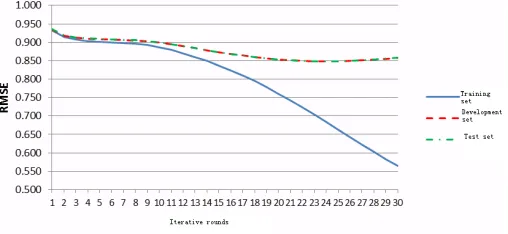
In the training process of the method based on gradient descent, the iteration is an important parameter. This study was designed to investigate the change of predicted performance of baseline model on the training set, development and test sets.
As the five experimental results are very similar, the experiment only describes the experimental results of one from 5 groups of data in order to analyze the impact on performance of iterative rounds. Since optimization criterion of the training algorithm is minimize the prediction error of training set. With the increase in the number of iteration, the prediction error (RMSE) of the training set is declining. When the iteration is too much ( in this experiment , the iteration count over 24 ), it began to appear over-fitting , prediction error of test set and development set start gradually increasing.
______________________________________________________________________________
It can be seen from Figure 3, that the change of properties of the test set and the prediction set is generally consistent. Therefore, fitting phenomenon can be predicted according to the change of the prediction error in the development set, and thus determine the iterative rounds of training.
4.3 THE EXPERIMENTAL IN THE EFFECT OF THE NUMBER OF IMPLICIT FACTOR ON THE PERFORMANCE
Experimental aims are to investigate the influence of the number of implicit factors on the performance of baseline model, and expect to find the number of implicit factors which can optimize model performance. Empirical parameters set of the baseline model is consistent with the previous experiment, and the iteration count is determined by the developer sets. The number of implicit factor k increases growth from 0 to 500, and the stepping in increase is 10. Figure 4 is an accurate indicating. Test set RMSE varies with the number of implicit factors.
As can be seen from Figure 4, when the number of implicit factor is 200, the performance of the model is close to optimal; if the number of implicit factor of the continue to increase the prediction performance of the model can hardly be improved.
When the number of implicit factor is 0, the model can not characterize the user preferences for items, and the prediction error is large. With the increase of the number of implicit factors, factors influencing the user preferences increase and the prediction error decreases. If the score data is the more perfect factors that models can describe sufficient enough of affecting, the more the number of implicit factor, factor model can describe the user preferences will be, and the higher the predictive performance is; However, in the case of limited training data, what fully data -driven implicit factor model approaches is the distribution of data itself. Therefore, when the number of hidden factors is large, continuing to increase the hidden factor can not further improve performance.
Figure 4 Baseline Model Performance (RMSE) Curve with the Implicit Number of Factors
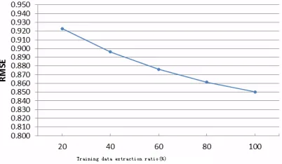
4.4 THE EXPERIMNTS IN THE EFFECT OF EXAMINING THE SIZE OF TRAINING DATA ON THE PERFORMANCE
[image:10.595.208.409.631.748.2]Experiment aims are to investigate the effect of the size of training data on the performance of the baseline model. The smaller the size is, the sparser the training data is. Experimental parameters of baseline model set is consistent with the previous experiment, the iteration count is determined by the development sets. The number of implicit factor k equals 200. The results in Figure 5 are the average experimental results which are corresponded by 5 groups of the same size of training data.
Figure 5 shows that the implicit factor model is sensitive to the training data scarcity. In this experiment, if 20% of the training data is only used, RMSE fell as much as 7.87 percent. The reason is that there is an essentially defect in implicit factor model: Learning implicit factor parameters through fully data-driven approach that may lead to over- match training data. In the learning process, what is constantly approaching is the distribution of the data itself, but not fully characterizes the user's preferences. When training data is sparse, the problem is more serious.
4.5 THE EXPERIMENT IN THE EFFECT OF MODEL EXAMINING THE INTEGRATION OF THE PERFORMANCE OF EXPLICIT AND IMPLICIT FACTORS
The goal is to validate the fusion of explicit and implicit factor model.
Baseline model is factor model which bias and the empirical parameters set is as follows: k=200,
γ =
0.005
,1 2 0.004
λ λ= = ,λ λ3= 4=0,denoted Baseline。
The experiment considers nine models of the integration of explicit and implicit factors, and introduce the following nine with correspondent features explicit factors in the model respectively: 18 movie -style , 3,208 actors, 706 directors, released Year ( 7 ), the two kinds of film color , 73 movies countries , 104 kinds of film language’s , the
user's age ( 7-segment ) and gender ( class 2 ) . Empirical parameters set of the model is as follows: k=200,
0.005
γ =
,λ λ1= 2=0.004,λ λ3= 4=0,λ λ5= 6=0.020,c=0.4。the first 8 models respectively denotedEFLFM-1, EFLFM-2, EFLFM-3, EFLFM-4, EFLFM-5, EFLFM-6, EFLFM-7, and EFLFM-8. The last model introduces all available 9 explicit factors and is denoted as EFLFM (Explicit Factor and Latent Factor Model).
Table 4 Relative to Enhance the Explicit and Implicit Integration Factor Model to Predict the Performance
Model RMSE Improvement (%)
[image:11.595.197.422.607.741.2]EFLFM 1.11
Table 3 Fusion Explicit and Implicit Factors in Prediction Performance Model
Model RMSE
Baseline 0.8502 EFLFM-1 0.8466 EFLFM-2 0.8439 EFLFM-3 0.8433 EFLFM-4 0.8419 EFLFM-5 0.8420 EFLFM-6 0.8418 EFLFM-7 0.8416 EFLFM-8 0.8410 EFLFM 0.8408
Tables 3 and 4 shows that after the introduction of these nine categories explicit factors in corresponding user features and articles feature, predictive performance of the model has been significantly improved. Experiment 4.3 has been verified, when the number of implicit factor of is more than 200, continuing to increase the implicit factor can hardly improve the performance. This proves the improvement of the model of explicit and implicit relative to the baseline model. It is not because of the increase of some factor dimensions but because of the introduction of an explicit factor. Experimental results show the adjustment of the structure of implicit factor model by introducing an explicit factor. Guiding the training process can ease over- training deficiencies of implicit factor and improve the forecast performance of the model .
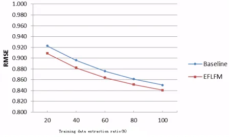
4.6 THE EXPERIMENT IN EXAMINING THE VARIATION OF THE PERFORMANCE OF THE MODEL AND WITH THE SIZE OF TRAINING DATA
Experiment aims are to validate the performance of the integration of explicit and implicit factor on different scale
training data. The smaller the size is, the sparser the training data. Figure 6 is the index curve model
RMSE
.______________________________________________________________________________
Experimental results show that the performance of the model of the fusion of explicit and implicit factor on the training data is significantly better than the implicit factor model. The smaller the size is, the higher the training data scarcity is and the more remarkable improvement it has. Introducing explicit factor can effectively alleviate the defects of the full data -driven implicit factor model is sensitive to sparse data.
CONCLUSION
This paper introduces implicit factor model with bias term as a baseline model and investigates the training iteration count. The number of implicit factor and the training data affect the performance for the baseline model through three sets of experiments. Completely data-driven factors could cause defects in the training data over match, the significance of explicit factors. On this basis, propose a fusion of explicit and implicit factor model and use the explicit factor to portray users’ demographic characteristics and content features of articles on the impact of user preferences. As to the defects in the training data over-match caused by the parameters using methods of fully data-driver implicit factor model. Finally, the validity of the model can be verified through experiments.
REFERENCES
[1]Linden G;Smith B,;York J, IEEE Internet Computing, 2003, 7(1):76-80.
[2]Koren Y;Bell R;Volinsky C, IEEE Computer, 2009, 4(8):30–37.
[3]GOLDBERG D ;NICHOLS D; OKI B, Communications of the ACM, 1992, 35(12):61–70.
[4]RESNICK P; LACOVOU N;SUCHAK M, et al, Grouplens: an open architecture for collaborative filtering of
netnews: proceedings of the ACM conference on computer supported cooperative work[C], New York, 1994:175-186.
[5]SARWAR B; KARYPIS G; KONSTAN J, et al, Item-based collaborative filtering recommendation algorithms:
proceedings of the 10th international conference on world wide web[C], 2001:285-295.
[6]CONNOR M; HERLOCKER J, Clustering items for collaborative filtering: proceedings of the ACM SIGIR
workshop on recommender systems[C],1999.
[7]XUE Gui-rong; LIN Chen-xi; YANG Qiang, et al, Scalable collaborative filtering using cluster-based smoothing:
proceedings of the 28th annual international ACM SIGIR conference on research and development in information retrieval[C], Salvador, Brazil, 2005:114-121.
[8]SARWAR B; KARYPIS G; KONSTAN J, et al, Application of dimensionality reduction in recommender
system—a case study: ACM WebKDD workshop[C], 2000.
[9]FUNK S. [OL].Available: http://sifter.org/~simon/journal/20061211.html.
[10]XIANG Liang; YUAN Quan; ZHAO Shi-wan, et al, Temporal recommendation on graphs via long- and
short-term preference fusion: proceedings of the 16th ACM SIGKDD interntional conference on Knowledge discovery and
data mining[C], New York, 2010:723-732.
[11]CHEN Tian-qi; ZHENG Zhao;Lu Qiu-xia, et al, Informative ensemble of multi-resolution dynamic
factorization models: KDD-Cup Workshop[C], 2011.
[12]BALABANOVIC M; SHOHAM Y,Fab: Communications of the ACM, 1997, 40(3):66-72.
[13]KRULWICH B, AI Magazine, 1997, 18(2):7-45.
[14]PARK S; CHU Wei, Pairwise preference regression for cold-start recommendation: proceedings of the third
ACM conference on recommender systems[C], New York, 2009:21-28.
[15]AGARWAL D; CHEN Bee-chung, Regression-based latent factor models: proceedings of the 15th ACM
SIGKDD international conference on Knowledge discovery and data mining[C], Paris, 2009:19-28.
[16]ZHANG Liang; AGARWAL D; CHEN Bee-Chung, Generalizing matrix factorization through flexible
regression priors: proceedings of the15th ACM conference on Recommender systems[C], Chicago, 2011:13-20.
[17]GANTNER Z; DRUMOND L; FREUDENTHALER C, Learning attribute-to-feature mappings for gold-start
recommendations: proceedings of the 2010 IEEE international conference on data mining[C], 2010:176-185.
[18]MANZATO G, Discovering latent factors from movies genres for enhanced recommendation: proceedings of