ECE-420: Discrete-Time Control Systems Homework 8
Due: Friday November 2
In this homework we will simulate and study the prediction full order observer coupled with state variable feedback, and then we will add on integral control. As you hopefully remember, having an integrator in our system is generally preferable to using a prefilter for achieving a zero steady state error for a step input, since it will help overcome errors in the plant model.
Some of the things we will do in this homework are a bit weird, but they are being done for the sake of demonstrating that your programs are working. Specifically, having the initial
estimates of the states so large is quite unrealistic, but it does allow us to see if the estimated states are converging to the true states. However, these initial large states force us to utilize very small closed loop poles for the state feedback and the integrators. Strange as it may seem, we need to use these small poles to keep the system from overwhelming the motor (having the control effort reach saturation).
For the all of these problems, utilize the torsional system models available from the class website that you used last week. This system should be sampled with Ts = 0.05.
(1 dof Integral Control)
1a) Copy your program DT_sv1_driver.m to a new file DT_sv1_servo_driver.m, then copy the Simulink file DT_sv1.mdl to DT_sv1_servo.mdl . Modify these new files to implement both state variable feedback and an integrator control . Your programs should be able to use either place or acker to place the closed loop poles directly. Note that if our system has an integrator in it, there should be no prefilter.
b) Modify the Matlab code (the poles and the place command) to place the poles of the closed loop system in such a way so that for a 15 degree step input, for the first disk:
• the settling time for your system is less than 1 s
• the percent overshoot for your system is less than 20% • the control effort does not hit a limiter (does not saturate) • the steady state error is zero
Simulate the system and turn in your graph.
(2 dof Integral Control)
2a) Copy your program DT_sv1_servo_driver.m to a new file DT_sv2_servo_driver.m, then copy the Simulink file DT_sv1_servo.mdl to DT_sv2_servo.mdl . Modify these new files to implement both state variable feedback and an integrator control. Your programs should be able to use either place or acker to place the closed loop poles directly. Note that if our system has an integrator in it, there should be no prefilter. Modify the Matlab code (the poles and the place command) to place the poles of the closed loop system in such a way so that for a 15 degree step input, for the first disk:
• the settling time for your system is less than 1 s
• the control effort does not hit a limiter (does not saturate) • the steady state error is zero
Simulate the system and turn in your graph.
2b) Repeat part a to control the position of the second disk. Turn in your graph.
(1 dof Full Order Observer)
3a) Copy your program DT_sv1_driver.m to a new file DT_sv1_observer_driver.m, then copy the Simulink file DT_sv1.mdl to DT_sv1_observer.mdl . Modify these new files to implement state variable feedback using a full order observer to estimate the states for a one degree of freedom system. Your programs should be able to use either place or acker to place the closed loop poles directly, or dlqr to place the poles using the LQR algorithm. Your programs should write all of the true states and all of the estimated states to the workspace. Note that if our system has no integrator in it, there should be a prefilter. Be sure u k( )is taken to be the signal just before the limiter.
3b) Modify DT_sv1_observer_driver.m to plot the first two true states (not the delayed control signal) and estimated states on the same graph, as well as the system output and the control effort.
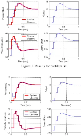
3c) Place both the state feedback and observer poles all at 0.5 (yes, this is a bad design) The output of the system is the position of the first disk and this is also the output available to the observer (C=Cyin this case). The disk is initially estimated to be at 5 degrees (be careful of units here! The model works in radians.). The initial estimates of the velocity and delayed control signal are zero. The real system starts at rest (all initial conditions are zero.) For a 10 degree step input you should get the graph shown in Figure 1. Turn in your plot.
3d) Now place the observer poles all at 0.3, then at 0.2, then at 0. Rerun the system and turn in your plots. You should see the estimated states converging mores quickly to the real states as the observer poles get closer to the origin.
Figure 1. Results for problem 3c.
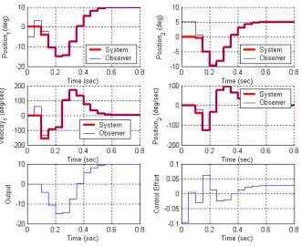
Figure 2. Results for part 3e.
(2 dof Full Order Observer)
4a) Copy your program DT_sv1_observer_driver.m to a new file
DT_sv2_observer_driver.m, then copy the Simulink file DT_sv1_observer.mdl to
[image:3.612.146.428.85.560.2]dlqr to place the poles using the LQR algorithm. Your programs should write all of the true states and all of the estimated states to the workspace. Note that if our system has no integrator in it, there should be a prefilter. Be sure u k( )is taken to be the signal just before the limiter.
4b) Modify DT_sv2_observer_driver.m to plot the first four true states (not the delayed control signal) and estimated states on the same graph, as well as the system output and the control effort.
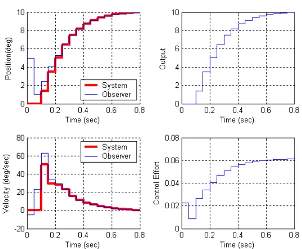
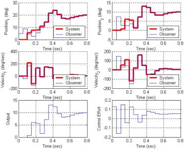
4c) Place all the state feedback poles at 0.2, and the observer poles at 0.06 0.08 0.1 0.12 0.14. You will probably need to use the place command to place the observer poles here. Assume the positions of both the first and second disk are available to the observer and the system output is the position of the first disk. The velocities of the disks and the delayed control signals are initially estimated to be zero. The estimated position of the first disk is assumed to be -5 degrees and the estimated position of the second disk is assumed to be 5 degrees. The real system is starts at rest. For a 10 degree step input you should get the graph shown in Figure 3. Turn in your plot.
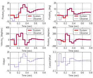
[image:4.612.122.452.351.621.2]4d) For the same conditions as part d, but assume the observer can only use the position of the second disk. You should get the results shown in Figure 4. Turn in your plot.
Figure 4: Results for problem 4d.
(1 dof Integral Control and Full Order Observer)
5) Now we want to combine the observer and state feedback with integral control for the one degree of freedom system. We will continue to utilize the torisional model we have been using.
5a) Copy your program DT_sv1_observer_driver.m to a new file
DT_sv1_obs_servo_driver.m, then copy the Simulink file DT_sv1_observer.mdl to DT_sv1_obs_servo.mdl . Modify these new files to implement both state variable feedback using a full order observer to estimate the states and integral control.
5b) Place all the state feedback poles at 0.4 and all of the observer poles at 0.2. The output of the system is the position of the first disk and this is also the output available to the observer (
y
Figure 5: Results for problem 5b.
(2dof Integral Control and Full Order Observer)
6) Finally, we want to combine the observer and state feedback with integral control for the two degree of freedom system. We will continue to utilize the torisional model we have been using.
6a) Copy your program DT_sv2_observer_driver.m to a new file
DT_sv2_obs_servo_driver.m, then copy the Simulink file DT_sv2_observer.mdl to DT_sv2_obs_servo.mdl . Modify these new files to implement both state variable feedback using a full order observer to estimate the states and integral control. Note that if our system has no integrator in it, there should be a prefilter. Be sure u k( )is taken to be the signal just before the limiter.