A transient boundary element method model of Schroeder diffuser scattering using well mouth impedance

A transient boundary element method 

model of Schroeder diffuser scattering 

using well mouth impedance

Hargreaves, JA and Cox, TJ

http://dx.doi.org/10.1121/1.2982420

Title

A transient boundary element method model of Schroeder diffuser 

scattering using well mouth impedance

Authors

Hargreaves, JA and Cox, TJ

Type

Article

URL

This version is available at: http://usir.salford.ac.uk/id/eprint/14625/

Published Date

2008

USIR is a digital collection of the research output of the University of Salford. Where copyright 

permits, full text material held in the repository is made freely available online and can be read, 

downloaded and copied for non­commercial private study or research purposes. Please check the 

manuscript for any further copyright restrictions.

A transient boundary element method model of Schroeder

diffuser scattering using well mouth impedance

Jonathan A. Hargreavesa兲and Trevor J. Cox

Acoustics Research Centre, The University of Salford, Manchester M5 4WT, United Kingdom

共Received 20 May 2008; revised 31 July 2008; accepted 19 August 2008兲

Room acoustic diffusers can be used to treat critical listening environments to improve sound quality. One popular class is Schroeder diffusers, which comprise wells of varying depth separated by thin fins. This paper concerns a new approach to enable the modeling of these complex surfaces in the time domain. Mostly, diffuser scattering is predicted using steady-state single frequency methods. A popular approach is to use a frequency domain boundary element method共BEM兲model of a box containing the diffuser, where the mouth of each well is replaced by a compliant surface with appropriate surface impedance. The best way of representing compliant surfaces in time domain prediction models, such as the transient BEM is, however, currently unresolved. A representation based on surface impedance yields convolution kernels which involve future sound, so is not compatible with the current generation of time-marching transient BEM solvers. Consequently, this paper proposes the use of a surface reflection kernel for modeling well behavior and this is tested in a time domain BEM implementation. The new algorithm is verified on two surfaces including a Schroeder diffuser model and accurate results are obtained. It is hoped that this representation may be extended to arbitrary compliant locally reacting materials.

©2008 Acoustical Society of America. 关DOI: 10.1121/1.2982420兴

PACS number共s兲: 43.55.Br, 43.20.Px, 43.20.Fn 关SFW兴 Pages: 2942–2951

I. INTRODUCTION AND OVERVIEW

Room acoustic diffusers can be used to treat critical lis-tening environments to improve speech intelligibility and to make music sound better.1Such devices are characterized by the uniformity of their scattering which may be measured under anechoic conditions,2a time consuming and expensive process. An alternative is to predict this dispersion using a numerical model, and the boundary element method共BEM兲 is well suited to this task.3 The speed and low cost of this approach aid prototyping of new designs and even allow automated optimization of treatments to be performed.4In a BEM model only the boundaries between obstacles and air are modeled as it is known how sound travels unobstructed. This produces smaller simpler meshes compared to volumet-ric methods such as finite element and finite difference time domain共FDTD兲. It also permits an unbounded volume of air to be modeled, making it ideal for free-field scattering sce-narios.

Most BEMs assume harmonic excitation so the un-knowns are time invariant and complex. While this fre-quency domain analyses is a useful tool, the transient behav-ior witnessed in the real world may only be recovered by solving many frequency domain models and then applying an inverse discrete Fourier transform共DFT兲. An alternative is to drop the time-invariant assumption and formulate the BEM in the time domain as is presented herein. This ap-proach was first published by Friedman and Shaw in 1962,5 however, its implementation is problematic and consequently the method is still not in widespread use in acoustics. Some of the key issues are outlined below.

A. Time domain BEM stability

The discretized boundary integral equations 共BIEs兲 forming the time domain BEM are typically solved by marching a solution on in time from known initial condi-tions, usually silence. However, being iterative this process has the potential for instability, a major impediment to the algorithm’s widespread use. Rynne6observed that similar in-stabilities affect all time domain BEM models regardless of the application, implying that this behavior is fundamental to the method rather than the problem considered.

The dominant analysis of this phenomenon is by the singularity expansion method.7 This expresses the system’s response to excitation as a sum of resonant poles, each with its own natural frequency and damping. In discrete time, each pole is a complex scalar describing the magnitude and phase change the corresponding mode undergoes in a time-step; hence a mode with a pole of magnitude greater than unity will grow and cause the solver to diverge. These dis-crete poles are closely related to the eigenvalues of the state-transition process which may be found numerically.8–10Such modes should be prohibited by the initial conditions, but in practice they can be seeded by numerical error in the solver; hence the onset of instability can appear highly random and implementation dependent. In addition, Rynne and Smith7 suggested that pole locations are perturbed by discretization error, so a pole of the BIE which is just stable may lead to a pole of the discretized system which is unstable.

When the problem of sound scattering from a body is stated as a BIE, the restriction that sound cannot travel through the body is lost and a continuation of the exterior medium, in this case, an air-filled cavity, is effectively cre-ated inside the body’s bounding surface. At certain

frequen-a兲_{Electronic mail: [email protected]}

cies, this cavity may resonate, storing energy so the time-invariant frequency domain BEM has a nonunique solution. In the time domain problem, these resonances correspond to oscillatory poles, borderline stable and likely candidates for corruption into divergence by numerical error. Such poles are not physically relevant so their removal is acceptable and improves solver performance. One method that achieves this in the frequency domain is the Burton and Miller formulation,11and has been transferred to the time domain as the combined field integral equation共CFIE兲.12

The BEM is a wave based method and its computational

cost increases rapidly with frequency. Acceleration

algorithms13,14have been published to address this issue but, as these are derived from the time-marching solvers for which instability issues remain, the focus herein remains on modeling smaller problems in a nonaccelerated fashion. In addition, some interesting work has been done on alternative solvers15–19that may be less sensitive to divergent poles than the current time-marching generation.

B. Modeling Schroeder diffusers

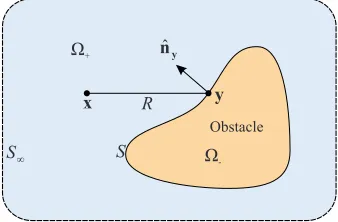
The class of diffuser considered in this paper is the phase grating diffuser, whose development can be traced back to the pioneering work of Schroeder.20,21 These com-prise a series of wells of differing depths according to a number theoretic sequence, separated by thin fins. Sound waves entering each well emerge following the time taken for them to travel to the bottom of the well, reflect, and travel back to the mouth. These delays are optimally decorrelated so the cumulative scattered sound is widely dispersed. Be-cause the wells store sound energy and then reradiate it, the scattered sound is diffused in both space and time; recently, this transient behavior has begun to attract research interest.22,23 In this paper, a one-dimensional diffuser based on the quadratic residue sequence will be considered; these are designed to diffuse in one plane only and take the form of an extruded cross section as depicted in Fig.1共a兲, where the fins are shown partially transparent.

Modeling the two sides of a thin fin aggravates an issue in the BEM known as thin shape breakdown.24This may be circumvented by using an open surface BEM which consid-ers the surface to be comprised of thin rigid plates. This formulation has previously been implemented in the time domain;25 however, it is unsuitable for modeling the solid part of the diffuser as it supports cavity resonances so is prone to instability.

Another modeling approach used in the frequency do-main, which avoids these issues, is to model the mouth of each well as a compliant surface; thus the mesh is simplified and becomes a box enclosing the device关Fig.1共b兲兴. A well’s behavior is described by the surface impedance of its mouth, a quantity ideal for use with BEM, which may be found by assuming that all propagation in the well is axial with negli-gible losses, so every point at the well mouth reacts locally. At first, this may seem unrealistic, but it has been numeri-cally shown to produce good results,26and Schroeder’s phase grating model makes these assumptions too. An equivalent time domain model is sought.

Differential boundary conditions may be used to model simple compliant materials such as broadband absorbers27,28 and limp membranes.29However, finding such from arbitrary surface impedance data is more complicated,30 although Drumm and Lam31 successfully fitted infinite impulse re-sponse filters to surface absorption data. It has been suggested32 that a convolution between waves traveling per-pendicularly into and out of the body may be a more robust approach; this is adopted for the application herein and found to be effective.

This paper is structured as follows: Sec. II introduces the boundary integral formulation of the scattering problem and the CFIE. Section III introduces the new time domain well mouth model and describes its substitution into the BEM. The discretization process and time-marching solver are specified in Sec. IV. Verification results are shown and dis-cussed in Sec. V followed by the conclusions in Sec. VI. Finally, details of the numerical integration procedure are outlined in the Appendix.

II. BOUNDARY INTEGRAL EQUATION FORMULATIONS

Figure2depicts a scattering problem, comprising an ob-stacle submerged in a connected medium ⍀+ with

equilib-rium density␳0which obeys the linear acoustic wave

equa-tion with speed of sound c.S is a surface conformal to the obstacle and sufficiently close that the obstacle’s surface properties may be ascribed to it; thus the obstacle resides in the interior domain⍀₋.S_⬁is the extent of the medium.xand

(a)

−1 −0.8 −0.6 −0.4

−0.2 0

0.2 0.4 0.6 0.8

1

−0.5 0 0.5 −0.6 −0.4 −0.2 0

x (m) y (m)

z

(m

) 0.2m

0.4m 0.1m

0.1m 0.4m

0.2m

[image:3.612.316.557.35.360.2]

(b)

y are the three-dimensional Cartesian vectors defining the observation and radiation points respectively,R=兩x−y兩is the distance between them, and nˆy is the surface normal unit vector aty.

Sound is represented by the velocity potential␸ which, while not a physical quantity, has the convenient property that both pressurep and particle velocityv may be derived from it:

p共x,t兲= −␳0␸˙共x,t兲, 共1兲

v共x,t兲=ⵜ␸共x,t兲, 共2兲

where t is the time and a dot above a quantity indicates temporal differentiation. An incident disturbance␸i共x,t兲 ex-ists in⍀+but does not reach the obstacle whilet艋0. When

␸i共x,t兲 does reach the obstacle, a wave ␸s共x,t兲 is scattered such that the total disturbance ␸t共x,t兲=␸i共x,t兲+␸s共x,t兲 matches the surface properties of the obstacle; thus this is an initial-boundary-value problem. Application of Green’s theorem33 allows the propagation of ␸s共x,t兲 in ⍀+ to be

stated as the Kirchhoff integral equation 共KIE兲 over its boundaryS艛S_⬁. In practice,S_⬁is chosen so distant that its contribution does not arrive within the modeling duration, so the integration domain may be reduced toS. This statement describes scattered velocity potential in a manner equivalent to the classical Huygens principle, being the propagation of the wavefront at each point on the boundary summed to-gether:

␸s共x,t兲=

冕冕

S

关␸t共y,t兲*nˆy·ⵜyg共R,t兲

−g共R,t兲*nˆy·ⵜy␸t共y,t兲dy兴. 共3兲

The term nˆy·ⵜy␸t共y,t兲 is the surface normal component of the particle velocity and is termed “normal velocity” for brevity. Despite the relation given in Eq.共2兲, normal velocity and velocity potential are independent fields on S since sur-face normal derivatives cannot be found from quantities only known on a surface.

*

denotes temporal convolution and g共R,t兲is the time domain Green’s function, which describes how sound travels from an instantaneous point source at t = 0 to a point observer at distanceR, given by

g共R,t兲=␦共t−R/c兲

4␲R , 共4兲

where␦共¯兲is a Dirac delta function. This delay term in the numerator encapsulates the finite propagation speed of sound, thereby dictating the domain of dependence of the scattered wave in Eq.共3兲and ensuring causality in the result-ing algorithm.

Consideration of the obstacle’s boundary condition at x

allows solution for the total surface sound, from which scat-tered sound at any desired off-surface point may be evalu-ated.

Specifically the CFIE is equivalent to the boundary con-dition共1 −␣兲pt共x,t兲=␣␳0cnˆx·vt共x,t兲when the limit is taken as x approachesS from the inside. The corresponding inte-gral operator may be expressed as

Lc兵␸t共x,t兲其=共1 −␣兲␸˙i共x,t兲+␣cnˆx·ⵜ␸i共x,t兲

= −

冋

共1 −␣兲⳵

⳵t+␣cnˆx·ⵜx

册

⫻

冕冕

S

关␸t共y,t兲*nˆy·ⵜyg共R,t兲

−g共R,t兲*_nˆy·ⵜy␸t共y,t兲兴dy ifx苸S−. 共5兲

This formulation is stated12to be the time domain equivalent to the Burton and Miller formulation11 commonly used in frequency domain acoustic BEMs. It differs slightly from the latter, in particular, with regard to the range of values taken by the real scalar blend parameter ␣, and matches more

closely its namesake in the electromagnetic BEM

formulation.34

When ␣=1₂ the boundary condition which founds the CFIE simplifies topt共x,t兲/nˆx·vt共x,t兲=␳0c, a condition

satis-fied by any plane wave propagating in the direction of nˆx, that is out of the cavity. More generally, it has been shown that when 0⬍␣⬍1 energy flows out of the cavity and it cannot support resonant modes.35 Consequentially, Lc has been shown to grant stability superior to alternate operators for a variety of test geometries. Therefore, it is desirable to derive the BEM algorithm from the CFIE for all compatible scattering obstacles.

III. WELL MOUTH SURFACE MODEL

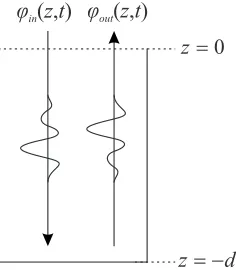
Consider a well of constant cross section and depthd, as depicted in Fig.3. It is assumed that the width of the well is small with respect to wavelength so that only axial plane wave propagation is supported. Accordingly, the sound in the well may be expressed as the superposition of two plane waves traveling into and out of the well, designated␸_inand

␸out. The rigid boundary condition at the base of the well

dictates that the incoming wave is reflected, such that the outgoing wave is the incoming wave with a fixed time delay. Under the assumption of time-harmonic oscillation

␸共z,t兲= Re兵e−i␻t_{⌽共z,␻兲其, the mouth of the well may be} char-acterized by this well known expression for surface imped-ance at the well mouth 共z= 0兲:

x

Ù+ nˆy

Ù

-Obstacle

y

R

S

[image:4.612.88.257.34.145.2]

S

FIG. 2. 共Color online兲A scattering problem comprising an obstacle sub-merged in a connected medium.Sis a surface conformal to the obstacle; hence the medium is said to be external toS.

Z共␻兲= Pt共0,␻兲 Vt,in共0,␻兲

=i␳0ccot共kd兲, 共6兲

wherek=␻c−1 is the wavenumber,Pt共z,␻兲is the total pres-sure, andVt,in共z,␻兲is the inward component of total particle

velocity. It is an ideal means of characterizing materials within a frequency domain BEM as it relates the two surface unknowns, pressure and normal velocity, by a complex scalar allowing the problem to be simplified to having only one surface unknown.

The same relationship may be stated in the time domain as pt共0 ,t兲=vt,in共0 ,t兲*z共t兲. However, a z共t兲 found by inverse

DFT of Z共␻兲 is typically noncompact in time and requires future values ofvt,in共0 ,t兲. This is due to the aggregation of

cause and effect in the quantities pt共0 ,t兲 and vt,in共0 ,t兲, and

means that this form cannot be used with a time-marching solver. Further to this, the inverse Fourier transform of Eq. 共6兲appears to be a nontrivial operation.

Another approach is to relate the incoming and outgoing

waves at the mouth of the well as ⌽_out共0 ,␻兲

=⌽_in共0 ,␻兲W共␻兲, where W共␻兲=ei2kd_{is the surface reflection} coefficient. This too may be stated in the time domain:

␸out共0,t兲=␸in共0,t兲*w共t兲, 共7兲

where the time-invariant surface reflection kernel w共t兲 is typically compact in time and expresses␸_outusing only past values of␸_in, hence is suitable for use with a time-marching solver. For the well model above,

w共t兲=␦共t− 2dc−1兲. 共8兲

Equations共7兲and共8兲will be used as the basis for the devel-opment of a time domain well mouth surface model.

A. Surface reflection boundary condition

Surface impedance is considered to vary spatially so

nˆx·ⵜ⌽t共x,␻兲= −i␻␳0⌽t共x,␻兲Z共x,␻兲−1holds for every point onS. Implicit in this is the assumption that the obstacle re-acts locally. An equivalent time domain boundary condition may be written using the surface reflection kernel form of Eq.共7兲:

␸out共x,t兲=␸in共x,t兲*w共x,t兲. 共9兲

The total velocity potential used in Sec. II is the sum of the incoming and outgoing waves:

␸t共x,t兲=␸in共x,t兲+␸out共x,t兲=␸in共x,t兲*关␦共t兲+w共x,t兲兴.

共10兲 This form suggests that␸in共x,t兲should be discretized as it is

the fundamental surface unknown and␸out共x,t兲 and␸t共x,t兲 are the secondary effects of its impingement on the obstacle. Similar statements may be found for total pressure and total normal velocity:

pt共x,t兲= −␳0␸˙t共x,t兲= −␳0

⳵

⳵t关␸in共x,t兲*关␦共t兲+w共x,t兲兴兴,

共11兲

nˆx·ⵜ␸t共x,t兲=nˆx·ⵜ关␸in共x,t兲+␸out共x,t兲兴

冏

= ⳵

⳵z关␸in共x,t+zc

−1_兲+␸

out共x,t−zc−1兲兴

冏

z=0

=1 c

⳵

⳵t关␸in共x,t兲*关␦共t兲−w共x,t兲兴兴. 共12兲 The above statements have been written without specifying w共x,t兲in anticipation that they may be capable of describing a broader class of scattering obstacle. For the welled rigid surface model discussed w共x,t兲=␦共t− 2c−1_{d共x兲兲, where}

d共x兲= 0 for rigid nonwell surfaces sections. The sifting prop-erty of the delta function is exploited to simplify the above:

␸t共x,t兲=␸in共x,t兲+␸in共x,t− 2c−1d共x兲兲, 共13兲

pt共x,t兲= −␳0关␸˙in共x,t兲+␸˙in共x,t− 2c−1d共x兲兲兴, 共14兲

nˆx·ⵜ␸t共x,t兲= 1

c关␸˙in共x,t兲−␸˙in共x,t− 2c

−1_{d共x兲兲兴. 共15兲}

These statements do not enforce that quantities are invariant over the cross section of the well as should be the case for plane waves; that restriction is left to the discretization scheme. Instead they state that the waves in the well are one dimensional, and that each point on the mouth of the well reacts locally. Radiation impedance of the well is accounted for in the boundary integral description of the problem. Sub-stitution into Eq.共5兲creates an operator that can calculate the sound scattered by an obstacle comprising rigid and welled sections while not supporting cavity resonances:

共1 −␣兲␸˙i共x,t兲+␣cnˆx·ⵜ␸i共x,t兲

=Lc兵␸in共x,t兲+␸in共x,t− 2c−1d共x兲兲其 ifx苸S−. 共16兲

In the following section, this new operator will be discretized to form a time-marching BEM.

IV. THE MARCHING-ON-IN-TIME METHOD

The surface quantities must be discretized in order for a solution to the boundary conditions onSto be found numeri-cally. As suggested by Eq.共10兲, to ensure compatibility with

0

=

z

d

z

=

[image:5.612.114.232.32.167.2]

-w

in

( , )

z t

w

out

( , )

z t

the new surface reflection boundary condition,␸in共x,t兲 will

be discretized in preference to the usual ␸t共x,t兲. Otherwise the discretization scheme follows that used in Ref. 12.

The surfaceSis partitioned intoNsflat elements denoted Sn, all small with respect to the anticipated spatial variation of the sound field, and time is discretized into Nt regular time-steps with duration ⌬t. Discretization of the incoming wave is achieved by approximating it by a weighted summa-tion of basis funcsumma-tions:

␸in共x,t兲=

兺

n=1

N_s

兺

_i

=1

N_t

wn,ifn共x兲Ti共t兲, 共17兲

wherewn,i are the discretization weights,

fn共x兲=

再

1 ifx苸Sn

0 otherwise

冎

共18兲

are the spatial basis functions, and

Ti共t兲=T共t−i⌬t兲 共19兲

are the temporal basis functions, the latter being regularly delayed copies of the mother basis function T共t兲. Currently T共t兲 is chosen to be the piecewise polynomial used in Ref. 12.

This discretization scheme is substituted into Eq. 共16兲 and the summations and weights are brought outsideLc. Col-location is performed in space and time to form a matrix equation; evaluation atxm共the center of elementSm兲 andtj =j⌬tcontributes a row to

Z₀wj=ej−

兺

l=1

⬁

Zlwj−l, 共20兲

where l=j−i is the retardation index and the weights wi;n =wn,i. The interaction matrices are defined as follows:

Zl;m,n=Lc兵fn共x兲Tj−l共tj兲+Tj−l共tj− 2c−1dn兲其, x=xm−,

共21兲

wherednis the well depth of elementSnand equals zero for rigid nonwell elements. These are evaluated efficiently and accurately by regularization to contour integrals and adaptive numerical integration; details are included in the Appendix. The excitation vectors are evaluated as

ej;m=共1 −␣兲␸˙i共xm,tj兲+␣cnˆx·ⵜ␸i共xm,tj兲. 共22兲

This algorithm is commonly referred to as the marching on in time 共MOT兲 or “retarded potential” algorithm and intu-itively possesses an iterative structure with sound traveling from element to element with a finite speed. It may more generally be considered to be a matrix solver between exci-tation coefficients and discretization weights, which exploits a pattern in the interaction matrices due to the regular tem-poral basis functions.

Discretization accuracy may be quantified spatially and temporally by considering the maximum frequency ␻_max present in the incident wave. The maximum phase variation over an element with largest dimension⌬xin a time-step is

␻max共⌬t+⌬xc−1兲. The logical assumption that spatial and temporal discretization error should be of similar magnitudes

suggests the choice ⌬x⬇c⌬t, as favored by Bluck and Walker.8 This leads to nonzero off diagonals in the matrix

Z0, necessitating a matrix solution at each time step.Z0will

in practice be very sparse and an iterative matrix solver seeded with the previous time-step’s weights provides an ef-ficient implementation.

In the following section, the new time domain well mouth surface model will be verified against frequency do-main BEM implementations.

V. RESULTS

The new algorithm implements a time domain BEM model of a welled obstacle characterized by the new surface reflection boundary condition. This has required develop-ment of the integration scheme but the numerical machinery is otherwise as previously published. Verifying this algo-rithm’s results will demonstrate that the new surface reflec-tion boundary condireflec-tion is performing correctly.

Verification is achieved by comparison with frequency domain BEM implementations which have previously been shown to accurately match experimental data.36Two scatter-ing problems are considered, both of which involve obstacles possessing wells, the first being an object with uniform depth wells covering one face and the second being a Schroeder diffuser. A harmonic point source illuminates the surface for sufficient duration that the system reaches steady state and any instability has the opportunity to appear. The DFT is applied to the time domain data and the error versus the frequency domain BEM is quantified at the frequency of excitation. Using single frequency excitation is clearly an uninspiring application of the time domain BEM but is being done purely to achieve rigorous verification.

Two frequency domain BEM implementations are used. The closed body version models the well mouths as surface impedances according to Eq. 共6兲. The open body version is capable of modeling the thin fins separating the wells so that the wells are modeled explicitly.

One mesh is used for each surface, and the time domain BEM is verified for a wide range of time-step durations de-fined by their relationship to spatial resolution, denoted im-plicitness c⌬t⌬x−1. This is done because time-step duration has been associated with stability in many publications; evi-dently different values affect whether poles are perturbed into divergence. For each of these, a far-field harmonic point source, located 100 m distant normal to the obstacle, excites the system at a frequency such that the number of time-steps per excitation period␤= 2␲共⌬t␻兲−1 assumes a range of pre-determined values. For each combination, the error e be-tween the time and frequency domain BEMs is calculated from the normalized mean complex difference between the respective source-to-collocation-point transfer functions at the excitation frequency:

e共␻兲=兺m=1 N_{s 兩}

HTD共xm,␻兲−HFD共xm,␻兲兩

兺m=1

N_{s 兩}

H_FD共xm,␻兲兩

. 共23兲

In the frequency domain, the transfer functionH_FDis simply the total pressure divided by the source monopole pressure:

HFD共x,␻兲=

Pt共x,␻兲 Psource

. 共24兲

In the time domainHTDis found by division of the DFT of

the total velocity potential by the DFT of the source mono-pole potential:

HTD共x,␻兲=

F兵␸t共x,t兲其共␻兲 F兵␸source共t兲其共␻兲

. 共25兲

The first 50␤共defined below兲iterations are omitted from the DFT to allow the time domain solution to reach steady state. The next 100␤ iterations are chosen for DFT; this length maintains periodicity and eliminates windowing error. This error ratio is displayed for each integration type as a percent-age contour plot between time-step implicitness and tempo-ral resolution␤.

A. Uniform welled body

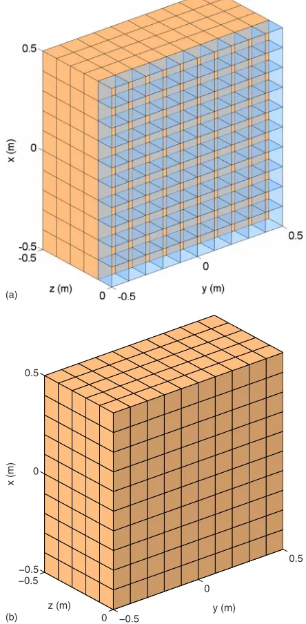
This body is a box 1.0 m2 by 0.5 m deep and its front face is covered by a lattice of wells all 0.1 m deep. Figure 4共a兲shows the open surface mesh comprising 580 thin plate elements, and Fig.4共b兲shows the equivalent surface imped-ance mesh comprising 400 elements; the thin elements are partially transparent and the well mouth elements are colored darker. ⌬x= 0.1 m for both meshes. The surface impedance model requires roughly half the memory and computation time required by the thin plate model.

Figure 5shows the error between the time domain and frequency domain models of the mesh in Fig. 4共b兲 versus time-step implicitness and temporal resolution. To the left of the figure where the time-step duration is explicit, spatial resolution is poor with respect to excitation wavelength so the accuracy of all BEM suffers. Toward the bottom of the figure, temporal resolution of the excitation frequency is poor; error here primarily originates from the time domain BEM. However, in the middle to upper right quadrant of the figure, discretization error is low and good agreement occurs. No instability is witnessed for any time-step duration indi-cating that the CFIE operator has successfully avoided sup-porting any cavity resonances even when combined with the new well mouth surface model.

Figure 6 shows the interference patterns that occur be-tween incident and scattered sound as further evidence that the well mouth surface model is behaving as expected. The receivers are arranged in a vertical line that starts behind the obstacle 共left of the figure兲, passes through its center, and emerges at the front 共right of the figure兲. They are spaced such that none touches the surface. The magnitude of the source to receiver transfer function H is plotted in decibel versus the receiver z coordinate. Data series are shown for the surface impedance mesh关Fig.4共b兲兴modeled by the time domain BEM 共TD impedance兲 and the frequency domain BEM for closed surfaces 共FD impedance兲, and for the thin plate mesh 关Fig. 4共a兲兴 modeled by the frequency domain BEM for open surfaces共FD thin plate兲. The vertical lines at z= 0.0 and z= −0.5 indicate the front and back of the ob-stacle and the shaded area indicates the wells of the mixed mesh. Time-step duration was chosen such that⌬x=c⌬t.

Interference effects between the incident and scattered waves are evident in front of the surface and in this region there is excellent agreement between the time and frequency domain algorithms. The BEM for open surfaces is seen to extend the interference patterns into the welled region and its surface normal gradient approaches zero as expected from the rigid well floors. Inside the surface, the frequency do-main BEM for closed surfaces achieves the best cancellation, but the results still confirm that the time domain surface reflection response boundary condition does not permit sound to flow into the cavity. In the shadow region behind the obstacle, all models, roughly agree but there is no appar-ent interference behavior.

This modeling problem has shown excellent stability and agreement with a verified frequency domain BEM on a simple surface with welled sections. A more complex real-world device will now be modeled.

(a)

−0.5

0 −0.5

0

0.5 −0.5

0 0.5

y (m) z (m)

x

(m

)

[image:7.612.324.546.40.492.2]

(b)

B. Quadratic residue diffuser

This device modeled has a design wavelength of 1.4 m, a well width of 0.3 m, a height of 1.0 m and follows the quadratic residue depth sequence关2 4 1 0 1 4 2兴. A diagram of the real device and the equivalent surface impedance model were shown in Figs. 1共a兲 and 1共b兲, respectively. ⌬x = 0.1 m for both meshes giving them 972 and 792 elements, respectively; consequentially, the surface impedance model requires roughly two-thirds of the memory and computation time of the thin plate model.

The relationship between the quadratic residue diffuser

共QRD兲meshes does not exactly mirror that between the uni-form welled body meshes. Specifically, the well mouths of the surface impedance model mesh have been discretized into elements with the same spatial resolution as the rigid parts of the surface; this is a standard technique used to mesh compliant surfaces in the frequency domain. Each element reacts locally which is equivalent to having the wells parti-tioned by a lattice structure similar to that present on the front face of Fig.4. This is not quite equivalent to either the

real device, the model in Fig. 1共a兲, or Schroeder’s plane wave model, but it has been shown to produce reasonable results.3

Figure7shows the error between the time and frequency domain implementations of the surface impedance model of the QRD depicted in Fig.1共b兲. It is plotted versus time-step implicitness and temporal resolution. The trends are the same as observed for the uniform welled surface, with universal stability and good agreement in the upper right quadrant, indicating that the new algorithm is functioning correctly. The first modal frequency along the wells of the QRD

共171.5 Hz, ␭= 2 m兲 is indicated by a dashed line and in-creased error can be observed close to it. This was an unex-pected result since the well mouth impedance model effec-tively partitions the well, and its significance is an ongoing research question.

Figure8 shows the magnitude of the source to receiver scattered sound transfer function in decibel versus receiver angle relative to the surface normal. This is calculated ac-cording to Eqs.共24兲and共25兲with the modification that scat-tered pressure and velocity potential are used in place of their total sound counterparts. The 91 receivers are uniformly spaced in a 5 m radius arc located in the primary scattering plane of the QRD. Data series are shown for the surface impedance mesh 关Fig. 1共b兲兴 modeled by the time domain

1% 1% 2% 2% 2% 3% 3% 5% 5% 10% 10% 10% 10% 30% 30% 30% 30% 30% 30% 30% 50% 50% 50% 00%

log₁₀(c∆t/ max∆x)

β

−15 −0.8 −0.6 −0.4 −0.2 0 0.2 0.4 0.6 0.8 1 10

[image:8.612.57.295.32.206.2]

15 20

FIG. 5. Error between time and frequency domain BEMs for closed surfaces both modeling the uniform welled surface.

−2 −1.5 −1 −0.5 0 0.5 1 1.5 2

−120 −110 −100 −90 −80 −70 −60 −50 z (m) |H| (dB) TD impedance FD impedance FD thin plate

FIG. 6.共Color online兲Total receiver sound though the uniform welled sur-face at 202 Hz⬅␤= 12. The vertical lines indicate the front and back of the obstacle and shading the wells on its front face.

1% 1% 2% 3% 3% 5% 5% 10% 10% 10% 10% 10% 10% 10% 30% 30% 30% 30% 30% 30% 30% 30% 30% 30% 30% 30% 50% 50% 50% 50% 50% 50% 50% 00%

log₁₀(c∆t/ max∆x) β

−15 −0.8 −0.6 −0.4 −0.2 0 0.2 0.4 0.6 0.8 1 10

[image:8.612.317.557.32.206.2]

15 20

FIG. 7. 共Color online兲Error between the time and frequency domain BEM for closed surfaces on the surface impedance model of the QRD. The dashed line indicates the first modal frequency along the wells of the QRD.

[image:8.612.54.293.533.703.2]

−100dB −90dB −80dB −70dB −90° −45° 0° 45° 90° TD impedance FD impedance FD thin plate

FIG. 8. 共Color online兲Scattered sound共dB兲at a receiver arc 5 m from the QRD at 202 Hz⬅␤= 12.

[image:8.612.316.556.588.713.2]

BEM 共TD impedance兲 and the frequency domain BEM for closed surfaces共FD impedance兲, and for the thin plate mesh

关Fig.1共a兲兴modeled by the frequency domain BEM for open surfaces 共FD thin plate兲. Time-step duration and excitation frequency were chosen such that⌬x=c⌬tand␤= 12.

Agreement between the models is good, though it is rec-ognized that the figure has a broad range of scale and unlike Fig.7 does not consider phase agreements. Despite the fact that this frequency is slightly below the design frequency of the diffuser 共245 Hz兲 some grating lobe behavior is visible and predicted by all models. Cancellation of incident and scattered waves at the scattering nulls 共⬇⫾70°兲 is more complete for the frequency domain results, mirroring the trend inside the body of the uniform welled surface共Fig.6兲, suggesting that the frequency domain algorithms are more accurate for time-harmonic problems.

This modeling problem has shown excellent stability and agreement with verified frequency domain BEMs for a geometrically complex real-world acoustic device. In the ap-plication of welled surfaces, the surface reflection boundary condition is achieving in the time domain what surface im-pedance achieves in the frequency domain.

VI. CONCLUSIONS

The investigation sought to transfer the technique of modeling the well mouths of a Schroeder diffuser as compli-ant surfaces from the frequency to the time domain. A direct inverse Fourier transform of surface impedance is unsuitable as its convolution kernels are typically noncompact in time and requires future data not available to a time-marching solver. Instead the response of the well to an incoming wave was described by its convolution with a time-invariant kernel denoted surface reflection response, which for a well is ex-tremely compact in time and only requires past data. Pres-sure and normal velocity at the mouth of the well are readily found from the incoming velocity potential so this was dis-cretized in preference to the more usual choice of total ve-locity potential. The new surface model was implemented and the algorithm verified on two welled surfaces, one of which was a Schroeder diffuser. Agreement with previously verified frequency domain BEM implementations was good. It is hoped that with further research this surface model may be generalized to include other classes of compliant obstacle currently modeled as locally reacting surface imped-ances in the frequency domain. One obstacle is the absence of data for the surface reflection response model when the obstacle is too complex to be considered analytically. Third octave averaged absorption coefficients are usually measured and quoted for most materials, and do not contain enough data to directly reconstruct the surface reflection kernel; in-stead some form of estimation is required. Drumm and Lam31and Fung et al.32 have both suggested approaches to replacing the convolutions appearing in FDTD surface mod-els with simple filters fitted to the absorption data, and their approaches may also be effective for time domain BEM. Further potential lies in the application of modeling materials with nonlinear and variant properties, for which time-harmonic models do not exist.

ACKNOWLEDGMENTS

This project was been funded by the UK Engineering and Physical Sciences Research Council 共EPSRC兲 under Grant No. GR/P01144/01.

APPENDIX: NUMERICAL EVALUATION OF INTERACTION COEFFICIENTS

Accurate evaluation of the interaction coefficients de-fined in Eq.共21兲is fundamental to the accuracy and stability of the algorithm. The temporal basis function chosen has discontinuous derivatives which cause discontinuities and delta functions in the surface integrands, making them un-suitable for solution by Gaussian integration. In addition, the integrand is singular so element self-interaction need often be considered as a special case.

The implementation herein exploits the flat elements and piecewise-constant spatial basis functions to permit regular-ization of all integrands by coordinate transformation,25,37 such that the collocation point is no longer a special case. The radial component of integration is performed analyti-cally, leaving the remaining numerical integration a one-dimensional contour integral. This allows an adaptive nu-merical integration scheme to be used, specifically Simpson integration with Romberg extrapolation. An absolute termi-nation criterion was used, meaning that larger more signifi-cant interaction coefficients were evaluated with higher pre-cision than smaller less significant ones. This process is arbitrarily accurate, has better computational cost scaling than two-dimensional integration, and allows the same inte-gration routine to be used for all element pairs as effort is automatically concentrated where necessary.

In order to clarify the conversion of the surface integral overSninto nested integrals two new coordinate systems will be used; one is a Cartesian system共v,w,z兲and one a cylin-drical polar system共r,␪,z兲, both shown in Fig.9. The origin and positivezdirection are the same in both coordinate sys-tems. The origin is defined as the projection of the colloca-tion pointxinto the plane ofSnand the positivezdirection is specified by nˆy. The positive v direction is defined as the projection ofnˆxinto the plane ofSn, such thatwˆ ·nˆx= 0. The positive theta direction is defined such that v=rcos共␪兲 and w=rsin共␪兲in the conventional way. The variablezrefers for thezcoordinate of the collocation pointxand any reference tov,w,r, or␪ implies the integration pointy.

The interaction coefficients are now evaluated according to the following expression, being the sum of integrals over the edges ofSnand a contribution from the origin:

wˆ vˆ

r

y x

R

0,0,z

x

y

n z ˆ

ˆ

x

nˆ

y

nˆ

, ,0

0 , ,

r

w v

y

n

S

Origin

[image:9.612.354.518.33.106.2]

Zl;m,n= 1 4␲edges

兺

冕

0

1

再

冋

冉

1 −␣−␣nˆx·nˆy z R

冊

d␪

d␮+␣nˆx·vˆ 1 R

dw d␮

册冋

冉

z

R− 1

冊

T˙j−l

冉

tj− R c

冊

+

冉

z

R+ 1

冊

T˙j−l

冉

tj− R+ 2dn

c

冊

册

+␣c

R

冋

nˆx·nˆy

冉

1 − z2

R2

冊

d␪ d␮+nˆx·vˆ

z R2

dw

d␮

册冋

Tj−l

冉

tj− R

c

冊

+Tj−l

冉

tj− R+ 2dn

c

冊

册

冎

d␮

−␪origin

4␲

冋

1 −␣−␣nˆx·nˆy z

兩z兩

册冋

冉

z

兩z兩− 1

冊

T˙j−l

冉

tj−

兩z兩 c

冊

+

冉

z

兩z兩+ 1

冊

T˙j−l

冉

tj−

兩z兩+ 2dn

c

冊

册

共A1兲

Numerical integration is with respect to ␮, a dimensionless edge position coefficient varying from zero at the start vertex to one at the end vertex. For an edge ethe partial differen-tials between this and the geometric integration variables are found as follows, where r_⬜is the minimum共perpendicular兲 distance from the origin to the line of edgee:

d␪ d␮=

兩e兩r_⬜

r2 sign共eˆ ·␪

ˆ_{兲, 共A2兲}

dw

d␮=wˆ ·e, 共A3兲

␪origin is the angle the edges of Sn make around the origin. This is zero if the origin is outsideSn and 2␲ifSncontains the origin. If the origin lies on an edge,␪_originwill equal the enclosed angle, intersection of one edge implies ␪_origin=␲, and intersection of a corner implies ␪_origin will equal the acute angle between the adjoining edges.

1_{P. D’Antonio and T. J. Cox, “Diffusor application in rooms,” Appl.}

Acoust.60, 113–142共2000兲.

2_{Audio Engineering Society Inc., “AES information document for room}

acoustics and sound reinforcement systems—Characterisation and mea-surement of surface scattering uniformity,” J. Audio Eng. Soc. AES-4id-2001共r2007兲.

3_{T. J. Cox and Y. W. Lam, “Prediction and evaluation of the scattering from}

quadratic residue diffusers,” J. Acoust. Soc. Am.95, 297–305共1994兲. 4_{T. J. Cox and P. D’Antonio,Acoustic Absorbers and Diffusers 共Spon,}

London, 2004兲.

5_{M. B. Friedman and R. P. Shaw, “Diffraction of pulses by cylindrical}

obstacles of arbitrary cross section,” ASME J. Appl. Mech.29, 40–46

共1962兲.

6_{B. P. Rynne, “Instabilities in time marching methods for scattering}

prob-lems,” Electromagnetics6, 129–144共1986兲.

7_{B. P. Rynne and P. D. Smith, “Stability of time marching algorithms for}

the electric field integral equation,” Electromagn. Waves4, 1181–1205

共1990兲.

8_{S. J. Dodson, S. P. Walker, and M. J. Bluck, “Implicitness and stability of}

time domain integral equation scattering analysis,” ACES. J.13, 291–301

共1998兲.

9_{P. D. Smith, “Instabilities in time marching methods for scattering: cause}

and rectification,” Electromagnetics10, 439–451共1990兲.

10_{H. Wang, D. J. Henwood, P. J. Harris, and R. Chakrabarti, “Concerning}

the cause of instability in time-stepping boundary element methods ap-plied to the exterior acoustic problem,” J. Sound Vib. 305, 289–297

共2007兲.

11_{A. J. Burton and G. F. Miller, “The application of integral equation}

meth-ods to the numerical solution of some exterior boundary-value problems,” Proc. R. Soc. London, Ser. A323, 201–210共1971兲.

12_{A. A. Ergin, B. Shanker, and E. Michielssen, “Analysis of transient wave}

scattering from rigid bodies using a Burton–Miller approach,” J. Acoust. Soc. Am.106, 2396–2404共1999兲.

13_{A. A. Ergin, B. Shanker, and E. Michielssen, “Fast analysis of transient}

acoustic wave scattering from rigid bodies using the multilevel plane wave time domain algorithm,” J. Acoust. Soc. Am.107, 1168–1178共2000兲. 14_{A. E. Yilmaz, J.-M. Jina, and E. Michielssen, “A fast Fourier transform}

accelerated marching-on-in-time algorithm for electromagnetic analysis,” Electromagnetics21, 181–197共2001兲.

15_{G. C. Herman and P. M. van den Berg, “A least squares iteratively}

tech-nique for solving time-domain scattering problems,” J. Acoust. Soc. Am. 72, 1947–1953共1982兲.

16_{Y. Shifman and Y. Leviatan, “On the use of spatio-temporal}

multiresolu-tion analysis in method of moments solumultiresolu-tions of transient electromagnetic scattering,” IEEE Trans. Antennas Propag.49, 1123–1129共2001兲. 17_{Y. K. Chung, T. K. Sarkar, B. H. Jung, M. Salazar-Palma, Z. Ji, S. Jang,}

and K. Kim, “Solution of time domain electric field integral equations using the Laguerre polynomials,” IEEE Trans. Antennas Propag. 52, 2319–2328共2004兲.

18_{Z. Ji, T. K. Sarkar, B. H. Jung, M. Yuan, and M. Salazar-Palma, “Solving}

time domain electric field integral equation without the time variable,” IEEE Trans. Antennas Propag.54, 258–262共2006兲.

19_{S. Barmada, “Improving the performance of the boundary element method}

with time-dependent fundamental solutions by the use of a wavelet expan-sion in the time domain,” Int. J. Numer. Methods Eng. 71, 363–378

共2007兲.

20_{M. R. Schroeder, “Diffuse sound reflection by maximum-length}

se-quences,” J. Acoust. Soc. Am.57, 149–150共1975兲.

21_{M. R. Schroeder, “Binaural dissimilarity and optimum ceilings for concert}

halls: More lateral sound diffusion,” J. Acoust. Soc. Am.65, 958–963

共1979兲.

22_{A. Farina, “A new method for measuring the scattering coefficient and the}

diffusion coefficient of panels,”86, 928–942共2000兲.

23_{J. Redondo, R. Picó, B. Roig, and M. R. Avis, “Time domain simulation of}

sound diffusers using finite-difference schemes,”93, 611–622共2007兲. 24_{R. Martinez, “The thin-shape breakdown共TSB兲of the Helmholtz integral}

equation,” J. Acoust. Soc. Am.90, 2728–2738共1991兲.

25_{Y. Kawai and T. Terai, “A numerical method for the calculation of}

tran-sient acoustic scattering from thin rigid plates,” J. Sound Vib.141, 83–96

共1990兲.

26_{T. J. Cox and Y. W. Lam, “Prediction and evaluation of the scattering from}

quadratic residue diffusers,” J. Acoust. Soc. Am.95, 297–305共1994兲. 27_{T. Ha-Duong, B. Ludwig, and I. Terrasse, “A Galerkin BEM for transient}

acoustic scattering by an absorbing obstacle,” Int. J. Numer. Methods Eng. 57, 1845–1882共2003兲.

28_{P. H. L. Gronenboom, “The applications of boundary elements to steady}

and unsteady potential fluid flow problems in two and three dimensions,” Appl. Math. Model.6, 35–40共1982兲.

29_{R. P. Shaw, “Diffraction of acoustic pulses by obstacles of arbitrary shape}

with a robin boundary condition,” J. Acoust. Soc. Am. 41, 855–859

共1967兲.

30_{C. K. W. Tam and L. Auriault, “Time-domain impedance boundary}

con-ditions for computational aeroacoustics,” AIAA J.34, 917–923共1996兲. 31_{I. A. Drumm and Y. W. Lam, “Development and assessment of a finite}

difference time domain room acoustic prediction model that uses hall data in popular formats,” Proceedings of Internoise, Turkey, 2007.

32_{K.-Y. Fung, H. Ju, and B.-P. Tallapragada, “Impedance and its}

time-domain extensions,” AIAA J.38, 30–38共2000兲.

33_{A. D. Pierce, Acoustics: An Introduction to Its Physical Principles and}

Application共McGraw-Hill, London, 1981兲.

34_{D. A. Vechinski and S. M. Rao, “Transient scattering from dielectric}

cyl-inders: E-field, h-field and combined-field solutions,” Radio Sci.27, 611– 622共1992兲.

35_{D. J. Chappell, P. J. Harris, D. Henwood, and R. Chakrabarti, “A stable}

boundary integral equation method for modeling transient acoustic radia-tion,” J. Acoust. Soc. Am.120, 74–80共2006兲.

36_{T. J. Cox and Y. W. Lam, “Evaluation of methods for predicting the}

scat-tering from simple rigid panels,” Appl. Acoust.40, 123–140共1993兲. 37_{Y. Ding, A. Forestier, and T. Ha-Duong, “A Galerkin scheme for the time}