Mobility-aware IMU-based Energy Efficient Routing
Protocol for UWSN
Muhammad Tayyab1,2*, Abdul Hanan Bin Abdullah1, Mohd. Murtadha Bin Mohamad1
1School of Computing, Universiti Teknologi Malaysia, Johor Bahru, Malaysia 2HITEC University, Taxila, Pakistan
Received August 19, 2019; Revised October 27, 2019; Accepted October 29, 2019
Copyright©2019 by authors, all rights reserved. Authors agree that this article remains permanently open access under the terms of the Creative Commons Attribution License 4.0 International License
Abstract Underwater Wireless Sensor Network
(UWSN) is one of the promising technologies having a wide range of applications, which includes underwater natural resources exploration, marine life study and underwater pipeline monitoring. Due to the harsh underwater environment, it is very challenging to provide an energy-efficient mobility-aware routing protocol for data collection. Due to the regular movement of the water currents, it becomes difficult to design a routing protocol that manages mobility of sensor nodes without the need of the localization details and with minimum energy utilization. Another issue of the UWSN is how to efficiently detect and avoid void nodes in a void area. The effect of the void node during routing increases energy utilization of the sensor nodes, which leads to decrease in the network lifetime and packet delivery ratio.In this paper, a Mobility-aware IMU-based Energy Efficient Routing (MIER) protocol for UWSN has been proposed to address issues including i) higher transmission overhead due to flooding of localization information exchange ii) and void node occurrence that leads to higher energy utilization and packet loss. The opportunistic data forward approach has been employed for the node communication. Extensive simulation has been carried out and the results show that MIER outperforms existing related research work in terms of end-to-end delay, packet delivery ratio and network lifetime.Keywords
UWSN Routing, Mobility Management, Void Node Handling, IMU-based Routing1. Introduction
Underwater acoustic sensor networks have been recommended as an effective technology for the support of aquatic applications ranging from environmental monitoring to intrusion detection [1]. Normally in underwater, acoustic networks are large number of mobile
sensor nodes, which are often deployed in a region of interest to shape a network for an investigation. In such networks, each node is equipped with various sensors like environmental sensor(s), positioning system, acoustic modem, active/ passive mobility system. Surface sinks are equipped with acoustic, radio modems and GPS [2]. In a multi-sink environment, each sensor node forward sensed data to any one of the sinks with an acoustic hop-by-hop or multi-hop routing named anycast routing [3]. The destination sinks transfer data to a central data headquarter for processing purpose through wireless communication. The communication path between source and sink nodes keep changing due to the water currents [4]. The network topology is highly dependent on water currents. Due to this phenomenon, nodes require localization information exchanging. In addition, void node is created due to the phenomenon, in which there is no further path available towards sink in most of the recent studies, reactive measures are usually employed in handling void node area, meanwhile, in the proposed solution the void node area is managed right from node deployment and before packet forwarding, which in turn guarantees packet delivery and reduces energy utilized.
Due to non-functioning of the GPS in an underwater environment, the localization technique becomes very difficult to accomplish [2]. Since the underwater channel is severely limited by bandwidth, broadcasting periodic routing updates to maintain routing path is also an expensive procedure.
(𝑧𝑧) 𝑎𝑎𝑎𝑎𝑎𝑎𝑎𝑎 and ignore other two 𝑎𝑎𝑎𝑎𝑎𝑎𝑎𝑎 which are (𝑎𝑎) 𝑎𝑎𝑎𝑎𝑎𝑎𝑎𝑎 and (𝑦𝑦) 𝑎𝑎𝑎𝑎𝑎𝑎𝑎𝑎. The continuous water current is the major cause of change in the network topology of the UWSN. Hence, the routing path need to be updated regularly and accordingly based on the mobility of the nodes.
In view of the existing approaches, the latest research works in the underwater networks intend to achieve localization-based routing, since there is no need for path maintenance or exchanging link-state information [4]. For the sake of clarity, it is significant to take into consideration that the proposed routing solution is centered on hop-by-hop routing from the sensors at the seabed to any sink on the sea surface. Thus, depth information and accelerometer are employed for the hop-by-hop-based routing.
The major drawback faced by the pressure-based routing is that, nodes do not know their network structure. Hence, the nodes makes localized path routing decisions without information on the availability and movement direction of their various neighbor nodes [7]. However, in terrestrial routing techniques, for example in DSDV and OLSR, each node in the network has an overall knowledge of the network structure that helps in efficient routing via shortest paths and easy routes maintenance. Thus, there is a strong relationship between route discovery and route maintenance in localization-based networks. These approaches lead to dead node or lower network lifetime. In order to propose an energy efficient protocol for UWSNs with mobility, the following related questions are aimed to be answered in this paper.
i) How to estimate mobility of UWSN nodes considering water current movement with minimum energy utilization.
ii) How to address high overhead caused due to flooding of localization information exchanging, which lead to higher energy utilization.
iii) How to estimate node movement towards a void area and avoid using it as a forwarding node, which causes packet loss and lower network lifetime.
Consequently, based on the aforementioned research questions, the following contributions of this paper have been highlighted as follows.
i) A mobility-aware routing protocol that augments neighbor node position estimation with minimum energy utilization in UWSN has been proposed. ii)To further improve on the network lifetime by
minimizing the energy utilization, an opportunistic directional data forwarding algorithm to avoid and prevents the occurrence of void nodes in UWSNs has been explored
iii) An estimation strategy for nodes moving to the void area is explored and presented.
iv) In addition, the proposed scheme is simulated and benchmarked in order to assess it performance against the closely related existing research work.
The remaining sections of the paper are structured as follows; Considering Section 2, a qualitative related literature on energy efficient routing in UWSNs have been revisited. Section 3, critically highlights the introductory concept of the MIER protocol with details of the design and development of the proposed MIER protocol for UWSN with minimum energy utilization have been presented. In section 4, simulation setups, simulation results analysis, and protocol benchmarking have been explicitly analyzed and discussed, followed by conclusions made in Section 5.
2. Related Work
In this section, related literatures have been qualitatively revisited considering various routing techniques for underwater WSN. Some detailed reviews on current advancements of UWSNs routing techniques have been presented in the following survey papers [1], [8]–[10]. There are two major routing techniques in the underwater WSN routing including location-aware and non-location-aware routing. However, this paper focuses on the non-location-aware routing techniques. The non-location-aware routing is categorized into pressure-aware routing and beacon-aware routing. The details of the reviewed literatures are presented the following subsections.
2.1. Non-Location-aware UWSN Routing
In this type of techniques, a forwarding node in the network does not employ the complete location information for choosing a suitable next forwarder for data forwarding in the routing process. Instead, actual distance, depth of node, hop count and layering are utilized for selecting optimal next forwarder considering opportunistic routing. The non-location-aware routing technique is divided into beacon-aware and pressure-aware routing techniques [11]. The related literature has been discussed in the following subsections.
2.1.1 Beacon-aware UWSN Routing
routing for underwater sensors has been suggested in [12]. A novel architecture has been presented based on super nodes. The super nodes work in such a way that they have direct connection with the sink node at the surface of the water, while the normal node is placed at the base of the water. By using beacon messaging considering different transmission power, the supper nodes partitions their area into different layers. Hence, choosing optimal based on layer ID. In another study, an adaptive power controlled routing scheme has been suggested to address high energy consumption in multi-hop routing based on underwater WSNs. The scheme employs different signal power degree and allocate to nodes in different layers closer to the sink nodes. The scheme works based on two phases, including layer assignment and data communication phases. The layer assignment phase involves layer formation and node selection within the layer, while the data communication involve forwarding of the underwater data from the base of the water to the top of the water that is, the sink node [13]. Consequently, several works have been carried out in this technique. However, in this research study we focus on the pressure-aware routing, which is discussed in the next subsection.
2.1.2 Pressure-aware UWSN Routing
In pressure-aware UWSN routing, the depth information and some other parameters including distance and direction of node are considered. These parameters can be measured locally using the inbuilt pressure sensors. Thus, this technique considers the realistic behaviors of the underwater WSN. Because sensors can move due to water current hence can change direction and move in-depth due to floatation [14]. The detailed discussions of the related literatures in pressure-aware routing techniques have been presented in this section. In order to minimize energy consumption of the underwater sensors, several protocols have been proposed. Pompili, et al. [15] proposed a routing protocol that considers end-to-end packet delivery and collective acknowledgments for effective routing in such a way that energy consumption of the sensor is minimized. Also, Vector-Based Forwarding (VBF) protocols that employ node location information in order to estimate a vector angle for forwarding a packet to the nodes present in the angle between the source and destination have been suggested in [10]. These techniques are employed to reduce energy consumption. However, due to the effects of continuous water currents, the topology changes hence, voids area is created which need to be addressed in the routing algorithm [16]. Also, there are geographic routing techniques, which require complete localization information of a node for data forwarding in underwater environments [17], [18]. A routing protocol which estimates the pressure level at each node is then used as a packet forwarding parameter. The packets are forwarded based on opportunistic routing from the nodes at the seabed
towards the sinks at the water surface in a greedy manner [18]. The pressure-based routing protocol does not require expensive distributed localization process. In general, DBR lacks an efficient mobility management, data forwarding process and effective recovery process from local maxima, which lead higher energy consumption. Another opportunistic-based data forwarding approach has been proposed in Pressure Sensor-Based Reliable (PSBR) routing for efficient data forwarding in UWSNs [19]. The PBSR is a sender-based approach with consideration of different parameters including link quality evaluator (FLQE), sensor depth distance and residual energy for selection a forwarder. However, PSBR assumed that all nodes are static, hence does not consider the movement of nodes due to water currents. Therefore, it does not consider the occurrence of void node or void area in the UWSNs. Further, a solution that tries to minimize or avoid void based on pressure routing in UWSNs (VAPR) has been suggested in [10]. The VAPR protocol takes advantage of the pressure-based concept of geographical routing, which direct data packet to any available sonobuoy on the top of the sea considering depth information present in the pressure gauge. The void problem is addressed by considering depth information, sequence number and hop count. However, the considered parameters are not enough to estimate a void node or void area. Because, the change in position of nodes have not been put into consideration, which leads to lower network life, that is, higher energy consumption.
In HydroCast [18], the study is based on how to address the aforementioned drawbacks by enhancing the efficiency of the forwarding node selection method which maximizes greedy routing with minimum interference. However, the aforesaid protocols have not considered mobility management of the nodes without the uses of GPS-based localization information. The proposed protocol relies on hop-by-hop-based greedy forwarding with a forwarding node selection algorithm based on mobility management using IMU [20].
3. Overview of MIER Protocol
The MIER protocol comprises of three main phases namely, initialization phase, neighbor movement phase, and data forwarding phase. In the initialization phase, nodes are randomly deployed at different depths. Then the sink node broadcast a beacon consisting of depth information and sink hop count. The broadcasted beacon is forwarded up to the bottom node. Neighbor movement phase is an enhanced beaconing system, where each nodes’ beacon consists of additional information including the senders’ depth, hop count to the neighbor, sinks and the IMU information. During receiving of updated beaconing information from neighbors, each node updates its neighbor table accordingly.
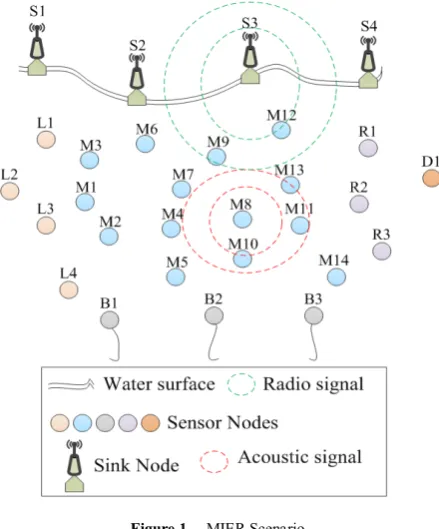
At the starting, initialization of variables is triggered by each surface sink and then starts beaconing. Once a node receives a beaconing message, the node compares it own depth with the senders’ depth to check whether the beacon is received from the nodes at the bottom depth of the sea or middle depth. Then, each node organize it neighbor nodes table to forward the data towards the surface sink. Normally, the direction of beaconing moves from the sink at the surface towards the deepest nodes at the seabed while packet forwarding is initiated from deepest nodes and target towards any of the sink at the surface. When multiple direction beacons are received from different sinks, the node with best direction towards the sink, which has the least hop count is selected for data forwarding. Then, a node that serves as next forwarder is selected based on the enhanced IMU-based beacons received by the sender node. For example, in Fig. 1, the beaconing process starts from sinks, node S1 – S4. All the decedent nodes receive beacon either directly from the sink or through beacon forwarding. Nodes on left edge of the network are named L1 – L4, nodes in the middle of the network are represented as M1 – M14, nodes on the right edge of network are named R1 – R3. While, the seabed or anchored nodes are depicted as B1 – B3 will get the forwarded beacon from upper nodes. Nodes that drift out initially soon after the deployment, D1, will not receive any beacon and will not be able to forward any since it is considered out of network.
Once the local state is updated, each and every node generate a beaconing message to be broadcasted to neighbors by increasing the number of hop count and providing information on it present depth, packet forwarding route direction, and the sequence ID number. This beaconing process will happen once in network lifetime to effectively construct hop-by-hop-based route towards the closest sink at the surface. Nodes on the left and right side edges of the network (L1 – L4, R1 – R3) have a tendency to drift out of the network with water currents. It is important to consider this fact in forwarding phase since it can create void node situation if drift happens. MIER consider this situation and maintain the potential void nodes in routing table by checking the IMU data of
[image:4.595.312.532.124.389.2]neighbor and comparing it with the current situation of that node. If a right node is drifted towards right that may create a void and vice versa for left edge nodes.
Figure 1. MIER Scenario
[image:4.595.315.532.542.730.2]In the underwater routing, one of the two scenarios must take place. The first scenario is when there exists no void area, the packets are routed directionally using greedy approach based on upward direction. Thus, the data forwarding direction can be fully relied on. The second scenario is when there is void area. Hence, this will lead to change of direction of data forwarding, and the next hop forwarding route direction. These are mutually employed to guide the routing path. For illustration purpose let assume the node R1 drifted to right and M12 drifted to the left side, thus a void area highlighted in Fig. 2.
The IMU inside R1 will trigger when it starts the drift to right edge of network. M13 and R2 were direct descendants of R1, they will receive the information and consider R1 out of network. Due to this change in network topology, the forwarding route M14 R3 R2 is now a void region, leaving the R2 as a local maxima and R3 trapped.
M12 is the middle node that drifted to left which still makes it a valid forwarder. M9 and M13 receive the information and add it to their routing table. The forwarding route for B3 node will be M14 M11 M13 M9 M12 S3.
[image:5.595.339.502.237.343.2]The following terminologies have been employed in the paper (see Fig. 2). A local maximum node is a node R2, which has shallowest depth level when compared to that of all its neighbor nodes however, it level is deeper compared to that of the sonobuoys; that is local Greedy Upward Forwarding (GUF) cannot perform any forwarding progress towards the sink at the sea surface. A trapped node defined as a node whose greedy forwarding path ultimately leads to a node called a local maximum. A local maximum node is the same as a trapped node, R3. As presented in the Fig. 2. A trapped node is often located below the curved-in area, which is situated in the void area. In addition, the area where trapped nodes are located is named as the trap area. The remaining nodes are called regular node, since they are not trapped. The detailed pseudocode of the different phases of MIER protocol is discussed in the following subsections.
3.1 Mobility-aware IMU-based Energy Efficient Routing Protocol
In this section, the pseudocode and flowchart of the MIER protocol are comprehensively discussed. One of the primary functions of MIER is to avoid the void regions in UWSN. There are two more important factors linked to neighbor node awareness. One is the edge nodes, which describes the right or left edge nodes of the network and secondly best optimal path towards the sink. MIER keeps record of neighbor nodes and then uses that information to check for nodes movement and watch on the nodes getting out of network for void node avoidance. This movement monitoring also helps in suggesting an optimal path towards the sink. MIER can be divided into three main phases from algorithm working point of view including the initialization, neighbor movement and data forwarding phase.
3.1.1 Initialization Phase
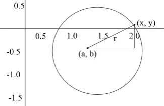
At this phase, every node triggers and tries to send its information to the neighboring nodes. This phase is utilized only at the start of network lifetime. Beaconing process is initiated by sinks. Each receiving node performs depth comparison to receive packets only from nodes above it. Then it calculates the estimated position by employing Eq. 1 and 2. The equations are the parametric form of equation
of a circle.
𝑎𝑎=𝑎𝑎+𝑟𝑟cos𝑡𝑡 (1)
𝑦𝑦=𝑏𝑏+𝑟𝑟sin𝑡𝑡 (2)
[image:5.595.303.541.440.748.2]Here 𝑎𝑎,𝑦𝑦 are the coordinates of neighbor node and 𝑎𝑎,𝑏𝑏 are the coordinates of current node, which is considered 0 in this case. The 𝑟𝑟 represents distance between the node itself and neighbor node. The alphabet 𝑡𝑡 represents the angle of arrival of forwarded packet. A simple diagram in Fig. 3, which illustrate an example of the trigonometric shape is as follows: for 𝑟𝑟= 1, with center value of (𝑎𝑎,𝑏𝑏) = (1.2,−0.5).
Figure 3. Illustration of Node Position in Trigonometric Shape.
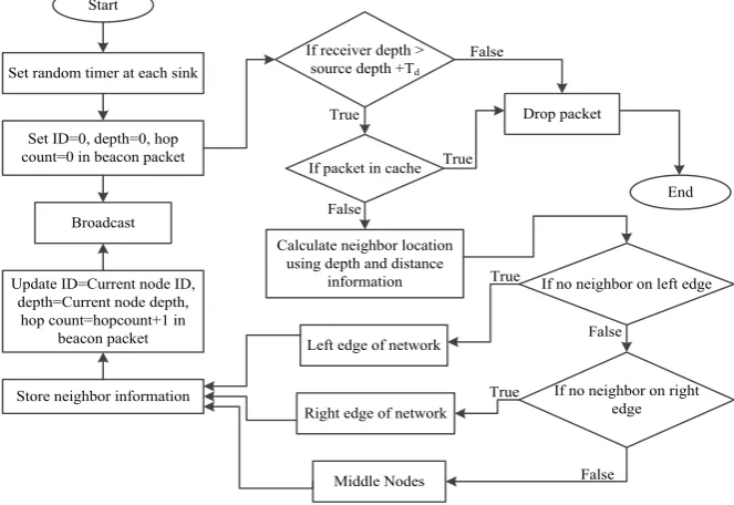
The pseudocode and flowchart of the initialization phase, which is carried out at the sink and receiver node are outlined.
Algorithm 1: Initialization Phase At sink node
1. Timer random value
2. ID 0, depth 0, hopcount 0 3. Broadcast packet
At receiver node (repetitive process till the bottom node) 1. If depth > source depth + Td then
2. If packet already in cache then 3. Drop packet
4. End if
5. Calculate neighbor relative location 6. If no left neighbor on source node then 7. Add neighbor as left edge of network 8. Else If no right neighbor on source then 9. Add neighbor as right edge of network 10. Else
11. Add neighbor as middle node of network 12. End if
13. Set ID current node ID 14. Set depth current node depth 15. Increment hopcount
16. Broadcast 17. Else
18. Drop packet 19. End if
0.5 1.0 1.5 2.0
(a, b)
.
r.
(x, y)
-0.5
-1.0
The first part of the Algorithm 1 is initialization at sink node, which involves the first line 1 to 3 of the pseudocode in the first part. The second part is the initialization of the receiver node with repetitive process until sink request get to the bottom node, which is from line 1 to 19 of the pseudocode. Next is the extensive flowchart of the initialization phase consisting of sink and the receiver node processes (see Fig. 4). After all nodes are updated through this process, each node store information of their neighbor nodes. This information consists of node ID, relative position and energy. This process is automatically iterated throughout the network, as each node becomes a beacon forwarding node as soon as it receives the beacon from previous one. The bottom nodes or the nodes closet to seabed will also forward the data further. However, since there is no deeper nodes in comparison and the receiver nodes above simply discard the packet because of depth comparison. As shown in algorithm 1, the forwarding cycle automatically ends once information is delivered to the sink node.
3.1.2 Neighbor Movement Phase
In this phase, the neighbor node movement algorithm pseudocode and flowchart are outlined. The neighbor movement phase is extensively discussed considering the node relative position changes, which lead to creation of void area. There is continuous movement in the network due to constant water currents. When a node is moved, the IMU inside a node generates a signal. This movement is assumed on 𝑎𝑎 − 𝑦𝑦 plane only. If the movement is beyond the threshold value, the node will broadcast a beacon with movement acceleration and direction information. At this event, neighbor nodes receiving the signal first perform the depth comparison to avoid storing information from nodes below. A data forwarding process can never happen on nodes below as the data is supposed to travel towards the sink, which is always above the sensing nodes. In case the node already contains neighbor information it will calculate the movement pattern by comparing IMU information with previously stored information about that specific neighbor. On the other hand, if the neighbor information is not already available, it means that a node is drifting towards current node coverage area. This will update the neighbors and the neighbor nodes will calculate the next best forwarding option based on previous scenario. The flowchart corresponding to the neighbor node movement phase has been depicted in Fig.5.
The first part of the Algorithm 2 is getting the movement magnitude at the inside water sensor nodes, which involves the line 1 to 5 of the pseudocode in the first part. The second part involves getting the node mobility of the receiver node, the process is from line 1 to 13 of the
algorithm. Next is the flowchart of the neighbor movement phase.
Algorithm 2: Neighbor Node Movement Phase
At moving node
1. Get movement magnitude from IMU 2. If movement magnitude > Tm then
3. Calculate movement direction and acceleration 4. Broadcast node and movement information 5. End if
At receiver node
1. If source node depth < current node depth then 2. If node not in neighbor table then
3. Add neighbor to routing table 4. End if
5. Calculate node distance and movement direction
6. If node is moving out of network then 7. Set void tag for source node 8. Else if node moving into the network then 9. Remove void tag for source node 10. Else
11. Drop packet 12. End if
13. End if
Algorithm 3: Data Forwarding Phase 1. Get data from sensor
2. Sort table by hop count in descending order 3. Select top energy nodes
4. If void node then 5. Select next
6. If no more nodes available then 7. No route possible
8. Else
9. Goto step 4 10. Endif
11. Else
12. Forward data to selected node 13. Set send counter
14. If send counter = 2 then 15. Goto Step 5 16. Else
17. Increment send counter 18. Endif
19. Endif
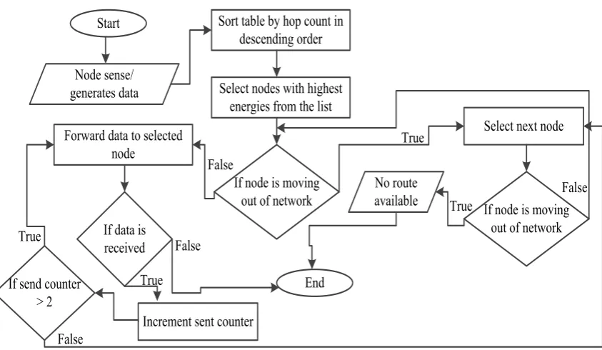
3.1.3 Data Forwarding Phase
[image:7.595.130.462.182.410.2]In this phase, the data forwarding Algorithm 3 pseudocode and flowchart are outlined. The whole process involved in the data forwarding phase are discussed. When source node generates data, it first selects the optimal neighbor node and forward the packet towards it. This process is repeated until the packet is handed over to any of the sink node. Neighbor node selection in MIER is simple as it already has the information of all neighbors with their movement pattern. MIER sorts the table according to lowest hop count and avoid the void nodes. It then selects the nodes with highest energy level out of the list to balance the energy consumption in network.
Figure 4. The Initialization Phase Flowchart
Figure 5. The Neighbor Node Movement Phase Flowchart
If receiver depth > source depth +Td Set random timer at each sink
Start
End Set ID=0, depth=0, hop
count=0 in beacon packet
Broadcast
Update ID=Current node ID, depth=Current node depth,
hop count=hopcount+1 in beacon packet
Store neighbor information
If packet in cache
Calculate neighbor location using depth and distance
information
Left edge of network
Right edge of network
If no neighbor on left edge Drop packet
Middle Nodes
If no neighbor on right edge
False False
True True
False
True True
False
Start Node movement
occur
If movement magnitude > threshold
False
True
Add to neighbor table Calculate node distance and movement direction
If node moving out of network
Set void tag with source node ID in routing table
If node is in neighbor table
If node is moving in network
Add node to routing table
Calculate direction and acceleration
Broadcast Neighbor receives
information
If neighbor depth < current node depth
Drop packet
Start False
False False
True
True
True
True
Figure 6. The Data Forwarding Phase Flowchart
The details of the systematic flow of the data forwarding algorithm has been depicted in Fig. 6. The subsequent section presents detailed procedure of the simulation implementation for the proposed protocol and obtained results analysis.
4. Simulation and Performance
Evaluation
The simulation setup and the outcome of the simulation carried out with result comparison to assess the performance of the proposed MIER protocol are presented in this section. The performance is assessed considering node movement in the underwater wireless sensor network for energy efficiency. Further, varied densities of the underwater sensor nodes have been employed to ascertain the scalability of the underwater sensor network. In the simulation, end-to-end delay, packet delivery ratio and network lifetime have been considered as the metrics for performance measurement. Average end-to-end delay, duration between the packet forwarding from first source to sink. Packet delivery ratio, ratio of total packets sent, and total packets received. Network lifetime, the time required to completely drain the battery of any node in the whole network.
The results attained are benchmarked with three baseline underwater protocols namely Mobile Sink–based Location Error–resilient Transmission Range (MMS-LETR) protocol [21], Pressure Sensor-Based Reliable (PSBR) routing protocol [19] and Weighting Depth and
Forwarding Area Division Depth Based Routing (WDFAD-DBR) [22] protocol. Further, the simulation environment setup is discussed in the following section
4.1 Simulation Setup
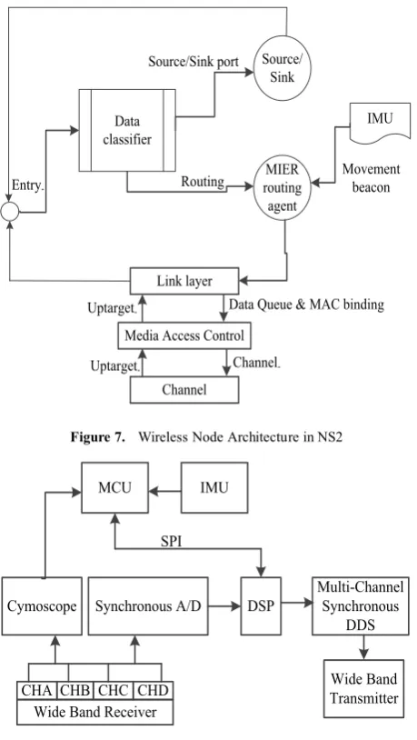
The proposed MIER protocol has been implemented using the AquaSim of the extended Network Simulator NS-2. Proof of concept and experimentation is performed in NS2. The underwater wireless node architecture of NS2 is shown in Fig. 7. There is an extension of NS2 called AquaSim specifically designed for simulating underwater sensor networks. AquaSim contains all basic tools to simulate an underwater sensor network. Since MIER utilizes an IMU, the node architecture is modified to accommodate it features. Fig. 8 shows the modified version of underwater node architecture. An IMU can generate two types of data i.e. acceleration and gyro (orientation). However, the MIER protocol utilizes acceleration data for simulation purpose, the gyroscope data from IMU are ignored.
Experimentation is done using random node deployment. The sensing area for UWSN is 800m x 800m x 800m. Each node is set at 100J initial energy. Node movement is set to random movement pattern with a variable speed of 0 to 2 m/s. Sample payload data packet size is set to 64 bytes. On top of it follows UDP protocol with random Constant Bit Rate (CBR) traffic. Table 1 shows the summary of simulation parameters and their corresponding values.
Start
Node sense/ generates data
Sort table by hop count in descending order
Select nodes with highest energies from the list Forward data to selected
node
If node is moving out of network If data is
received
Increment sent counter If send counter
> 2 End
No route available
Select next node
If node is moving out of network False
True
True False
True False
Table 1. Simulation Parameters Parameter Value
Grid size 800m x 800m x 800m Node speed 0 – 2 m/s Antenna type Omni directional Data packet size 64 bytes
Packet type UDP Traffic type CBR Physical channel Underwater channel Number of nodes 25 – 400
[image:9.595.306.543.186.373.2]The Fig. 7 and 8 depicts the NS-2 architecture and it functionalities, and underwater node architecture and it components relationship respectively.
Figure 7. Wireless Node Architecture in NS2
Figure 8. Functional Diagram of Underwater Node
4.4.2 Comparative Results and Discussions of MIER performance
In this subsection, the results are analyzed based on comparison with other existing related protocols. The experimental results attained for the proposed protocol with 95% confidence interval level have been presented in this section. Different metrics are employed including end-to-end delay, packet delivery ratio and network lifetime. The results for each of the metrics are depicted in Fig. 9 (a, b and c).
Figure 9(a). End-to-End Delay Based on Various Node Density
Fig. 9(a) represents the benchmarking of MIER with other related protocols including PSBR and MMS-LETR. PSBR has the highest delay because of its redundant data transmission, packet collision occurs much more often than any other protocol. This lead to high packet drop, high delay to send data to the sink and higher energy utilization. PSBR controls the packet flow by selecting the highest quality link channel. MMS-LETR follows the same technique. However, the void node handling is supported by their protocols, which decreases the delay. However, in their protocol void is detected after it has occurred, thus causing higher delay and higher energy utilization. Nevertheless, in the MIER protocol, the void area and node are avoided before data transmission, it provides the easiest shortest path towards the sink providing the lowest source node to sink delay, hence having lower energy utilization. Fig. 9(b) compares the packet delivery ratio among the protocols. The higher collision rate in PSBR lead to packet drop, which result to lowest packet delivery ratio with higher energy consumption. The PSBR has better route selection that increases the result of the packet delivery ratio. However, the void nodes are not efficiently handled in the PSBR protocol that leads to packet drop with higher energy utilization. PSBR and MIER both can handle void nodes. Nevertheless, MMS-LETR does not take the node movements into consideration. Thus, some packets are lost with either collision or sent to the nodes IMU
Source/ Sink
MIER routing
agent Data
classifier
Link layer
Media Access Control
Channel Routing Source/Sink port
Movement beacon Entry
-Uptarget
-Uptarget
-Data Queue & MAC binding
Channel
-MCU IMU
Cymoscope Synchronous A/D DSP Multi-Channel Synchronous DDS
CHA CHB CHC CHD Wide Band Transmitter Wide Band Receiver
SPI
0 1 2 3 4 5 6 7
150 200 250 300 350 400 450
End
-t
o-en
d d
el
ay
(s
ec
)
Number of Nodes
[image:9.595.60.290.294.701.2]drifting outside network. Interestingly, the proposed MIER protocol tackled the aforementioned limitations.
Figure 9(b). Packet Delivery Ratio Based on Various Node Density
Redundant transmissions in WDFAD-DBR reduces network lifetime significantly as shown in Fig. 9(c). Along with that, WDFAD-DBR selects same path repeatedly, which drops the energy of nodes within the specific path. PSBR selects the high quality path for data forwarding and take energy balancing into account that significantly increase performance compared to WDFAD-DBR.
The PSBR protocol works better only for lower number of nodes and works in contrast for higher nodes with lower network lifetime. VAPR does not uses any energy balancing technique and lower number of nodes create more void nodes which reduces the network lifetime. Both PSBR and MMS-LETR generate excessive network overhead in form control packet to maintain the path. The proposed MIER protocol in contrast, generates significantly lower control packets with energy balancing which results in increase in overall battery life of the nodes. Therefore, lower energy is dispensed and hence higher network lifetime is attained
Figure 9(c). Packet Delivery Ratio Based on Various Node Density
Based on the results obtained in all the metrics, it demonstrates that the proposed MIER protocol performs better than the existing baseline protocols for underwater wireless sensor network. The next section concludes the research works.
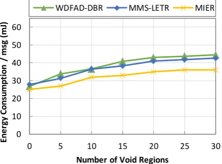
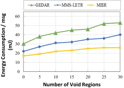
Energy consumption is also calculated while energy usage per message alongside different node density and different number of void regions are depicted in Figure 10(a), (b) and (c) respectively. The result of the proposed MIER against the baseline work including WDFAD-DBR and MMS-LETR has been observed. This observation is considered under different densities of the nodes and different number of void regions. The aim of employing the energy consumption as a metric for evaluation is to validate the MIER performance improvement in comparison with baseline research works. In addition, it also shows its behavior in different situations in terms of network lifetime, network scalability and dynamic network restructuring. The energy consumption is a metric employed to measure the average energy used per message per node. Energy consumption at each node may vary for each message however average energy consumption represents an overall value which indirectly shows the network lifetime and energy balancing.
Figure 10(a). Energy Consumption per message for various for large numbers of nodes
Figure 10(a) shows that the energy consumption of the MIER performs better against the two schemes GEDAR and MMS-LETR. GEDAR and MMS-LETR both utilize depth adjustment technology. In depth adjustment actively uses node propellers to move the node to a different depth. This is an energy intensive process. In addition, MMS-LETR increases the transmission power if the node is in a void region. This let MMS-LETR increase PDR however it adversely affects energy consumption. On contrary MIER let a node transmit beacon only when there is a potential void. This transmission happens within single hop range which in comparison is significantly energy efficient process. The average energy consumption per message by the schemes is 35.4 mJ, 27.1 mJ and 20.7 mJ for GEDAR, MMS-LETR and MIER respectively. The
0 0.1 0.2 0.3 0.4 0.5 0.6 0.7 0.8 0.91
150 200 250 300 350 400 450
PD
R
Number of Nodes
PSBR MMS-LETR
WDFAD-DBR WDFAD-DBR
0 10 20 30 40 50 60
0 5 10 15 20 25 30
Ene
rg
y C
ons
um
pt
io
n
/ m
sg
(m
J)
Number of Void Regions
WDFAD-DBR MMS-LETR MIER
0 5 10 15 20 25 30 35 40 45 50
150 200 250 300 350 400 450
Ene
rg
y
Co
ns
um
pt
io
n /
m
sg
(m
J)
[image:10.595.61.292.118.298.2] [image:10.595.312.530.379.534.2] [image:10.595.64.282.567.727.2]percentage of performance improvement of MIER against GEDAR and MMS_LETR are 41.5% and 23.7% respectively.
Figure 10(b). Energy Consumption for various numbers of void regions (nodes=250)
Figure 10(c). Energy Consumption for various numbers of void regions (nodes=400)
The Figure 10(b) and Figure 10(c) represent the average energy consumption comparison at the nodes alongside the number of void regions. From the result, a proportional correlation is observed between the energy consumption and number of void regions. Since there is no depth adjustment and communication adjustment technology used in MIER it performs better when compared to GEDAR and MMS-LETR. The average energy consumption by the schemes is 49.2 mJ, 32.2 mJ and 27.3 mJ for GEDAR, MMS-LETR and MIER respectively. The percentage of performance improvement of energy saving by MIER against GEDAR and MMS-LETR are 44.5% and 26.7% respectively.
5. Conclusions
In the underwater wireless sensor network, Water currents are constant and it keep changing the topology of the sensor node. Constant change in network topology and
nodes drifting changes the optimal forwarding routes and sometime create void regions. Hence, a change due to constant water currents is an important factor in route selection with minimum energy consumption. Taking continuous node movement into account during route selection positively affects in overall network performance. Thus, this article proposes MIER routing protocol, which exploits IMU sensor data to check node availability and movement. Unlike other protocols including GEDAR, WDFAD-DBR and PSBR, which calculate the routing route on a static scheme. The MIER protocol sends an automatic beacon based on node drift to its neighbors. This event based triggering system keeps the route updated and saves energy because of less network overhead. The extensive simulation demonstrates that the proposed MIER protocol outperforms the existing protocols by achieving lower energy consumption (network lifetime) with higher packet delivery ratio.
REFERENCES
K. M. Awan, P. A. Shah, K. Iqbal, S. Gillani, W. Ahmad, [1]
and Y. Nam, “Underwater Wireless Sensor Networks: A Review of Recent Issues and Challenges,” Wireless Communications and Mobile Computing, vol. 2019. Hindawi Limited, 2019.
A. Khan et al., “Routing protocols for underwater wireless [2]
sensor networks: Taxonomy, research challenges, routing strategies and future directions,” Sensors (Switzerland), vol. 18, no. 5, May 2018.
M. Sathish, K. Arumugam, and S. N. Pari, “Triangular [3]
metric based routing protocol for underwater wireless sensor network,” in 2017 2nd International Conference for Convergence in Technology, I2CT 2017, 2017, vol. 2017-January, pp. 1239–1245.
N. Javaid, A. Majid, A. Sher, W. Z. Khan, and M. Y. [4]
Aalsalem, “Avoiding void holes and collisions with reliable and interference-aware routing in underwater WSNs,” Sensors (Switzerland), vol. 18, no. 9, Sep. 2018.
A. Khasawneh, M. S. B. A. Latiff, O. Kaiwartya, and H. [5]
Chizari, “A reliable energy-efficient pressure-based routing protocol for underwater wireless sensor network,” Wirel. Networks, vol. 24, no. 6, pp. 2061–2075, Aug. 2018. M. T. Ali et al., “Dist-Coop: Distributed cooperative [6]
transmission in UWSNs using optimization congestion control and opportunistic routing,” Int. J. Adv. Comput. Sci. Appl., vol. 9, no. 6, pp. 356–368, 2018.
M. Z. Abbas, K. Abu Bakar, M. Ayaz, and M. H. Mohamed, [7]
“An overview of routing techniques for road and pipeline monitoring in linear sensor networks,” Wirel. Networks, pp. 1–11, 2017.
R. Bhardwaj Assistant Professor Daviet, J. Harpreet Kaur [8]
M-Tech Daviet, J. Rajeev Kumar, and A. Professor, “A Survey on Routing Protocols for the Underwater Wireless Sensor Network,” 2017.
0 10 20 30 40 50 60
0 5 10 15 20 25 30
En
erg
y C
on
su
m
pt
io
n
/ m
sg
(m
J)
Number of Void Regions
0 10 20 30 40 50 60
0 5 10 15 20 25 30
Ene
rg
y
Co
ns
um
pt
io
n /
m
sg
(m
J)
[image:11.595.76.286.130.282.2] [image:11.595.65.283.326.481.2]M. Tariq, M. ShafieAbd Latiff, M. Ayaz, Y. Coulibaly, and [9]
N. Al-Areqi, “Distance based Reliable and Energy Efficient (DREE) Routing Protocol for Underwater Acoustic Sensor Networks,” J. Networks, vol. 10, no. 5, May 2015.
Z. Rahman, F. Hashim, M. F. A. Rasid, and M. Othman, [10]
“Totally opportunistic routing algorithm (TORA) for underwater wireless sensor network,” PLoS One, vol. 13, no. 6, Jun. 2018.
S. Li, W. Qu, C. Liu, T. Qiu, and Z. Zhao, “Survey on high [11]
reliability wireless communication for underwater sensor networks,” J. Netw. Comput. Appl., p. 102446, Oct. 2019. J. Liu, M. Yu, X. Wang, Y. Liu, X. Wei, and J. Cui, “RECRP: [12]
An underwater reliable energy-efficient cross-layer routing protocol,” Sensors (Switzerland), vol. 18, no. 12, Dec. 2018.
P. Casari and A. F. Harris, “Energy-efficient reliable [13]
broadcast in underwater acoustic networks,” 2007, p. 49. R. W. L. Coutinho, A. Boukerche, L. F. M. Vieira, and A. A. [14]
F. Loureiro, “Geographic and opportunistic routing for underwater sensor networks,” IEEE Trans. Comput., vol. 65, no. 2, pp. 548–561, Feb. 2016.
D. Pompili, T. Melodia, and I. F. Akyildiz, [15]
“Three-dimensional and two-dimensional deployment analysis for underwater acoustic sensor networks,” Ad Hoc Networks, vol. 7, no. 4, pp. 778–790, 2009.
S. Basagni, C. Petrioli, R. Petroccia, and D. Spaccini, [16]
“CARP: A Channel-aware routing protocol for underwater acoustic wireless networks,” Ad Hoc Networks, vol. 34, 2015.
R. W. L. Coutinho, L. F. M. Vieira, and A. A. F. Loureiro, [17]
“DCR: Depth-Controlled Routing protocol for underwater sensor networks,” 2013 IEEE Symp. Comput. Commun., pp. 000453–000458, 2013.
N. Javaid et al., “Cooperative opportunistic pressure based [18]
routing for underwater wireless sensor networks,” Sensors (Switzerland), vol. 17, no. 3, Mar. 2017.
A. Latiff et al., “Pressure sensor based reliable (PSBR) [19]
routing protocol for underwater acoustic sensor networks Grid Computing View project Architectures for Optical Burst Switching Networks View project Pressure Sensor Based Reliable (PSBR) Routing Protocol for Underwate,” 2016.
J. H. Kepper, B. C. Claus, and J. C. Kinsey, “A Navigation [20]
Solution Using a MEMS IMU, Model-Based Dead-Reckoning, and One-Way-Travel-Time Acoustic Range Measurements for Autonomous Underwater Vehicles,” IEEE Journal of Oceanic Engineering, Institute of Electrical and Electronics Engineers Inc., 19-Jun-2018. M. Shah, Z. Wadud, A. Sher, M. Ashraf, Z. A. Khan, and N. [21]
Javaid, “Position adjustment–based location error–resilient geo-opportunistic routing for void hole avoidance in underwater sensor networks,” in Concurrency Computation, 2018, vol. 30, no. 21.
Z. A. Khan et al., “Region Aware Proactive Routing [22]