Variable and Fixed Structure Augmented IMM Algorithms Using Coordinated Turn Model

(1)

Variable- and Fixed-Structure Augmented

IMM Algorithms Using Coordinated Turn Model

Emil Semerdjiev

1

Ludmila Mihaylova

1

Bulgarian Academy of Sciences

Central Laboratory for Parallel Processing

‘Acad. G. Bonchev’ Str., Bl. 25-A, 1113 Sofia, Bulgaria

E-mail: [email protected], [email protected]

http://www.bas.bg/test/mmosi/MMSDP.html

X. Rong Li

∗

University of New Orleans

Department of Electrical Engineering

New Orleans, LA 70148

Phone: 504-280-7416, Fax: 504-280-3950

E-mail: [email protected]

1

Partially supported by the Bulgarian Ministry of Education and Science - Grant No. I-808/98

∗_{Research supported by ONR Grants N00014-97-1-0570 and N00014-00-1-0677, NSF Grant ECS-9734285, and LEQSF Grant}

(1996--99)-RD-A-32.

Abstract - A new variable-structure (VS) Augmented

Interacting Multiple Model (AIMM) technique is developed in the paper. Fixed-structure (FS) and VS AIMM algorithms using augmented constant velocity and augmented coordinated turn (ACT) models, are proposed. The ACT model includes the difference between the unknown current turn rate and its value assumed in the IMM models. Due to the estimated turn rate, significant self-adjusting abilities are provided to the designed AIMM algorithms, which give very good overall accuracy and consistency. Both AIMM algorithms are compared to a particular VS adaptive grid IMM algorithm. It is shown that the VS IMM algorithms possess better mobility, while the FS AIMM algorithm possesses better consistency. The VS AIMM algorithm provides the best estimation of the turn rate.

Keywords: IMM, adaptive estimation, target tracking, coordinated turn model

1 Introduction

The Interacting Multiple Model (IMM) algorithm is one of the most effective among the multiple model algorithms used to overcome the usually arising uncertainty about the states and parameters of dynamic systems [1,6,7]. Discretizing the continuous domain of the unknown control parameters, the system behaviour is considered as a sequence of system transitions among a finite number of known discrete system modes, differing by their particular control parameters. The discretization step of the uncertainty domain predetermines the number of IMM models, the estimation accuracy, and the required computational load, which may turn out to be unacceptably high in certain circumstances. That is why the question “how to decrease the IMM models’ number without significant loss of accuracy?” is considered in a number of issues. This question is especially topical for

IMM tracking with the coordinated turn (CT) model [1,2,4].

The CT model [1, 2, 4, 8, 9, 13] is widely applied in IMM tracking applications design. It describes target maneuvers performed with constant turn rate, at constant height (the case of civilian aircraft) [1, p.77-78]. For military aircraft the assumption that the turn rate is known is less natural and the domain of unknown turn rates is significantly larger. Often, a single CV model and a considerable number of CT models are usually implemented to design a tracker with a fixed structure (FS) IMM algorithm (IMM-CV/CT) [8, 9], capable to cover a wide range of maneuvers. As it is known the FS algorithm uses a predetermined fixed set of models [7]. The required computational load depends on the number of models.

A brief analysis of solutions decreasing the number of IMM-CV/CT models is presented in Section 2. FS IMM algorithms using augmented CT models (ACT) and variable structure (VS) IMM designs using standard or ACT models are applied for this purpose. Here, two new IMM-CV/CT algorithms are proposed and evaluated in Sections 3-5. The basic idea of the Augmented IMM (AIMM) algorithm is considered and a new VS AIMM algorithm is proposed in Section 3. Two particular FS and VS AIMM-ACV/ACT algorithms using single augmented CV (ACV) model and two ACT models are developed in Section 4. Applying Monte Carlo simulation in Section 5, these algorithms are compared to a VS IMM-CV/CT algorithm similar to those described in [4], for a particularly hard scenario. All investigated algorithms demonstrate very good performance. Finally, inferences and notes are given in Section 6.

2 IMM-CV/CT algorithms

(2)

x

_k

=

F

_CT

x

_k₋₁

+

Gv

_k₋₁

.

Its state vector

x

k

=

[

X

k

,

X

k

,

Y Y

k

,

k

]

'

includes aircraft Cartesian coordinates and their derivatives;

T

is the sampling interval; the scalar system noise is white and Gaussian,

νk

~

N

(

0 ,

Q

CT

)

. Matrices

F

CT and

G

have the form:

F

T T

CT =

− −



      



      

1 0 1

0 0

0 1 1

0 0

sin cos

cos sin

sin cos

ω ω

,

G

T

=













1 2

2

1 2

2

0

.

and

ω >

0

for counterclockwise turns.

The CT model is usually jointly implemented with the constant velocity (CV) model [1, 2, 4, 7-9] describing the uniform target motion:

x

k

=

F

CV

x

k−1

+

Gv

k−1,

where

F

T

CV =



    



    

1 0 0

0 1 0 0 0 0 1 0 0 0 1

.

The above models are often augmented to cover a large range of possible target maneuvers using minimal number of models. Wang, Kirubarajan and Bar-Shalom investigate three ACT models in [13]. They are obtained augmenting the standard CV and CT model by the unknown turn rate

ωk

, which is included in the state vector

x

k

[

X

Y Y

]

a

k k k k k

=

,

ω

', and it is no more considered as a control parameter. Then, the nonlinear ACT model is once expanded in a Taylor series up to first-order, and once more – up to second-order terms, to develop a respective extended Kalman filter (EKF). The third IMM-CV/CT algorithm uses the Kastella’s CT model version, which is implemented in a respective EKF, too. Each of the three designed standard IMM algorithms uses a single CV model and a single ACT model. It is finally noted, that the three algorithms yield similar performance.

Li and Bar-Shalom [8] have designed three other adaptive FS IMM-CV/CT algorithms for industrial application. The first one uses standard CV and CT models applying least squares turn rate estimation, but it does not possess sufficient capabilities to track systems, whose turn rate rapidly changes. Both versions of the second proposed algorithm use a single ACV and two or four ACT models. The turn rate is treated as a random variable with certain known expected value and variance. The maneuvering models correspond to different levels of

the above expected turn rates, respectively. The standard IMM algorithm configuration is modified with an instantaneous feeding of the expected turn rate to the maneuver model(s) after the ACV interaction step [8, p.193]. Both algorithms reduce the noise during the uniform motion while maintaining the estimation accuracy better than unfiltered raw measurements [8, p.186].

A VS IMM-CT/CV algorithm is proposed by Munir and Atherton in [9]. The CT model is decomposed along each axis in two independent models, and further augmented by the corresponding linear accelerations

X

and

Y

. The turn rate

ω

_k is calculated at each step as the magnitude of the acceleration divided by the target speed. The proposed algorithm outperforms the standard FS IMM-CV/CT algorithm, when the turn rate range is not fully covered by the standard IMM models.

Another, higher quality performance is reported in [4]. Attractive estimation accuracy and significant reduction of the computational load is achieved due to the application of the advanced variable structure (VS) IMM approach [5-7]. Introducing grids of turn rates it becomes possible to develop switching grid IMM (SGIMM) and adaptive grid IMM (AGIMM) algorithms using a single standard CV and two CT models. Their performance is compared to those of a standard FS IMM using a complete set of CT models, and the AGIMM algorithm performance is proven to be the best.

Summarizing the above survey, it may be stated that the simple inclusion of control parameters in the state model does not automatically provide improved IMM algorithm performance. As a rule, the control parameters included in the new state vector are initially set to values placed at the center of the former parameter domain [13]. Each time, when the system jumps into a new mode, such EKF starts its motion from this initially preset mode. Evidently, some period of time is needed to reach the new system mode, and this period is larger than the respective time needed to reach the new mode if non-collocating models are used. Because of this performance de-terioration, the above mentioned IMM algorithms have yielded place to the more efficient VS algorithms like the recently proposed VS IMM ones [4]. However, due to the “artificial” nature of the VS IMM algorithms, it is not easy to design appropriate particular parameter grids and switching rules for SGIMM or model management for AGIMM. Also it is difficult to develop efficient VS IMM algorithms in conditions far from the initially assumed. That is why the idea to apply new approaches combining the advantages of having the control vector estimated and the mobility of the VS IMM algorithms is topical. Applying the recently proposed Augmented IMM approach [10-12], FS and VS AIMM algorithms are proposed and investigated in the present paper.

(3)

3 FS and VS AIMM algorithms

The efficiency of the AIMM approach has been validated in [10-12]. It has been successfully applied in such important practical applications as maneuvering aircraft and maneuvering ship tracking [10,11], as well as for fault detection and parameter drift estimation [12]. Maintaining non-collocating models, it estimates the unknown control parameters. As a result it adequately follows the abrupt changes in the system behaviour using small number of augmented models.

3.1 Fixed-Structure Augmented IMM

Algorithm

To describe the idea of the AIMM algorithm let us consider the stochastic hybrid system:

(

) ( )

x

k

=

f x

k−1

p

k−1

+

g p

k−

v

k−

0

1 0

1

,

, (1)

( )

z

k

=

h x

k k

+

w

k, (2) where

x

k

nx

∈ℜ

is the system state vector estimated based on the measurement vector

z

k

nz

∈ℜ

in the presence of unknown vector of the true control parameters

p

k n_p

0

_∈ℜ

. The additive system and measurement noises

v

k nv

∈ℜ

and

w

k nz

∈ℜ

are mutually independent, white, Gaussian: ν_k ~ N

(

0,Q_k

)

and

w

k

~

N

(

0 ,

R

k

)

. Functions

f

,

g

and

h

are known and remain unchanged during the estimation procedure.

To estimate the difference (displacement)

∆

p

i k,

between the current true control parameters

p

k

0

and their values

p

_i fixed in the

i

-th IMM model, the system state model is augmented by the following simple set of equations:

∆

p

_{i k}_,

=

∆

p

_{i k}_, ₋₁, (

∆

p

_{i ,0}

=

0

). (3) The difference

∆

p

i k,

=

p

k

−

p

i

0

, (4) for all

i

must obey the restrictions

∆

p

i k,

+

p

i

∈

[

p_imin,p_imax

]

, providing given minimal and maximal separation distances between the models. They prevent possible models’ merge or displacements.

The augmented state and system noise vectors of the

i

-th augmented model (

i

=

1,

N

) is written as:

[

]

x

_{i k}a

x

_{i k}

p

_{i k} nx np

, ,

' , ' '

=

∆

∈ℜ

+ ,

ν

_{i k}a

[

ν

_{i k}

ν

_p

]

nν n

i k

p

, ,

' ' '

,

=

∈ℜ

+ .

In general, the new model is nonlinear:

(

)

(

)

x_{i k}a_, = fa x_{i k}a_, ₋₁,p_i +∆p_{i k}_, ₋₁ +ga p_i +∆p_{i k}_, ₋₁ v_{i k}a_, ₋₁, (5)

(

)

z

k

h

x

p

w

a i k a

i i k k

=

,

+

∆

,

+

. (6)

Functions fa(.), ga(.) and ha(.) are known and remain unchanged during the estimation procedure.

Further, the EKF equations are derived by linearization of models (5) and (6). Functions

f

a

(

x

i k, −1

,

p

i

+

∆

p

i k, −1

)

and

g

a

(

x

i k, −1

,

p

i

+

∆

p

i k, −1

)

are expanded in Taylor

series up to first-order terms around the filtered estimate

, /

x

i k k a

−1 −1; the function

h x

(

p

)

a

i k,

,

i

+

∆

i k, is expanded

up to first-order terms around the predicted estimate

, /

x

_{i k k}a ₋1 [2, 3]. The equations of the

i

-th EKF take the

form:

, / , / , ,

x

i k k

x

K

a

i k k a

i k a

i k

=

₋1

+

γ

, (7)

(

)

,

, / , / , /

x

i k k

f

x

p

a a

i k k a

i i k k

−1

=

−1 −1

+

∆

−1 −1 , (8)

(

)

γ

i k k a

i k k a

i i k k

z

h x

p

, , / , /

,

= −

₋1

+

∆

₋1 , (9)

(

)

P

_{i k k}a _i

f

_{x k}a

P

_{i k}a _k

f

_{x k}a

Q

_{i k}a

i i

, / , , / ,

'

,

−1

=

φ

−1 −1 −1 −1

+

−1, (10)

( )

S

_{i k}

h

_{x k}a

P

_{i k k}a

h

_{x k}a

R

_k

i i

, , , / ,

'

=

−1

+

, (11)

( )

K

i k

P

h

S

a

i k k a

x k a

i k

i

, , / ,

'

,

=

₋ −

1

, (12)

( )

P

i k k

P

K S

K

a

i k k a

i k a

i k i k a

, / , / , , ,

'

=

−1

−

, (13)

where

K

i k a

, is the filter gain matrix,

P

i k k a

, / and

Q

i k a

, are the estimation error covariance and system noise covariance matrices,

γ

_{i k}_, and

S

i k, are the filter innovation and its covariance matrix, the system and the measurement Jacobian are

f

x k a

i, −1

=

∂

f

(

x

p

)

∂

x

a

i k k a

i i k k i k k a

,

, −1/ −1

+

∆

, −1/ −1 , −1/ −1

and

h

_{x k}a

i,

=

∂

h x

(

)

∂

x

a i k k a

i k k a

, / −1 , / −1;

φi

≥

1

is the EKF fudge factor.

Obviously, such indirect inclusion of control parameters in the state vector makes them “manageable”. As it is mentioned in [8], in this case the estimation accuracy of these parameters is not very important, as far as the other state vector components estimates are of major interest. What is important is the correct and timely detection of the system maneuver and the fast response of the filter to this detection. For example, estimates

∆

, /

p

_{i k k}

(4)

3.2 Variable-Structure Augmented IMM

Algorithm

The FS AIMM algorithm can be easy transformed into a new VS AIMM algorithm by substitution of the constant vector of deterministic parameters

p

i with the random vector of control parameters

p

i k, −1. At the end of each

scan the last filtered model displacement

∆

, /

p

_{i k}₋₁_k₋₁ is used to correct the old vector of control parameters

p

_{i k}_, ₋₁:

p

i k,

p

i k,

p

i k, /k

=

₋1

+

∆

₋1 ₋1 (

p

i,0

=

p

i), (14) predicting in this way its new values. The new control vector must obey the restrictions

[

]

p

_{i k}_, ₋1

+

∆

p

_{i k}_, ₋1_/_k₋1

∈

p

_i_,min

,

p

_i_,max , for all

i

.

After the above operation, the model displacement

∆

, /

p

_{i k}₋₁_k₋₁ should be set to zero:

∆

, /

p

i k−1k−1

=

0

. (15)

Otherwise, it will be taken into account twice in the EKF equations. Because of the last correction (15), the EKF (7)-(13) starts at each scan with no initial model ment. The new model displacement (in fact, the displace-ment’s increment) is generated by eqn. (7), so a new control vector should be predicted again at the end of the scan.

The proposed new VS algorithm has better dynamics than its FS predecessor version. The vector

p

_{i k}_,

accumulates all estimated increments

∆

, /

p

_{i k}₋₁_k₋₁ of the

i

-th EKF, while the

i

-th EKF in the FS AIMM algorithm is adjusted by the standard IMM’s mixture

∆

, /

p

i k−1k−1, in

which the estimated dominant displacement is reduced due to the usual IMM models interaction.

Finally, it should be noted, that the proposed here new VS AIMM approach is general – it does not depend on the implemented system and measurement models. The new VS AIMM algorithm is an adaptive VS IMM algorithm using minimal number of models that self-adjust their location in continuous parameter domain.

4 AIMM algorithms using CT model

The designed here AIMM algorithm versions use a single ACV model and two ACT models for left-turn and right-turn motions. They are obtained incorporating the equation:

∆

ω

i k,

=

∆

ω

i k, −1,

into the standard CV and CT models. The difference between the current true turn rate

ω

_k0 and its value

ωi

fixed in the i-th model is denoted by

∆ω

_{i k}_,

=

ω

_k0

−

ω

_i (

i

=

1 2 3

, ,

). The FS AIMM control parameters

ωi

are

assumed constant:

ω

₁

=

ω

_max for left turns,

ω

₂

=

0

for uniform motion, and

ω

₃

= −

ω

_max for right turns.

The CV model has the form:

x

_{i k}a,

=

F

_CVa

x

_{i k}a, −1

+

G

_CVa

v

_{i k}, −1,

i

=

2

(16)

where

[

]

x

_{i k}a_,

X

_{i k}_,

,

X

_{i k}_,

Y

_{i k}_,

Y

_{i k}_, _{i k}_, '

,

=

∆ω

,

ω

_{i k}_,

=

ω

_i

+ ∆

ω

_{i k}_, ,

F

T

CV a

₌













1

0

1

0

1

0

1

0

1

,

G

T

CV a

₌













1 2 2 1 2 2

0

1

.

The i-th ACT model (

i

=

1 3

,

) has the form: X_{i k} X_{i k} X_{i k} i k T Y T

i k i k i k i k , , , , , , , ,

sin cos

= − + − − − − − − − − 1 1 1 1 1 1 1 1 ω ω ω ω , cos sin , , , , ,

X_{i k} =X_{i k}₋₁ ω_{i k}₋₁T−Y_{i k}₋₁ ω_{i k}₋₁T, (17)

Y_{i k} X_{i k} i k T Y Y T

i k

i k i k

i k i k , , , , , , , ,

cos sin

= − − − + + − − − − − 1 1 1 1 1 1 1 1 ω ω ω ω , sin cos , , , , ,

Yi k =Xi k−1

ω

i k−1T+Yi k−1

ω

i k−1T,

∆

_ω

∆

_ω

∆ω

i k,

=

i k, −1

+

v

i k, −1.

The purpose of the scalar turn rate noise

v

_{i k}∆ω_, ₋₁ is to take into account possible system maneuvers.

The system Jacobi matrix has the form:

(

)

f

x

F

M

a CT i k

i k,

=













×

ω

0

1 4

1

, for

i

=

1 3

,

, where:

M X T T T

Y T T T

k i k k

i k k i k k i k k i k k

i k k

i k k i k k i k k i k k

11 1 2 2 1 , , / , / , / , / , / , / , / , / , / , / cos sin sin cos = − − − + −

ω ω ω

ω

ω ω ω

ω

,

M21,k T Xi k k, / i k k, / T Yi k k, / i k k, / T

sin cos

= − _ ω + ω _,

M _k i k kT i k kT i k kT X

i k k

31 2 1 , , / , / , / , / , / sin cos

=

ω

− +

ω

+

ω

ω ω ω

ω

i k k i k k i k k i k k

i k k

T T T

Y , / , / , / , / , / cos sin − 2 ,

M41,k T Xi k k, / i k k, / T Yi k k, / i k k, / T

cos sin

= − _ ω − ω _.

It is also supposed that only position measurements are available, i.e.

z

k

=

Hx

k

+

w

k, where

H =  

 

  1 0 0 0 0 0 0 1 0 0

.

The measurement noise w_k is white Gaussian, with

( )

(5)

In the VS AIMM algorithm the new control parameter

ωi k

, is predicted at the end of the previous

k

−

1

scan upon the base of its last value

ωi k

_, ₋₁ and the last filtered estimate

∆

, /

ω

i k−1k−1 (which is later set to zero) :

ω

i k,

ω

i k,

ω

i k, /k

=

−1

+

∆

−1 −1.

5 Simulation results

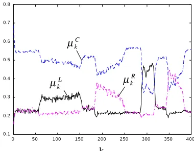
Both AIMM algorithms are compared to a particular implementation of the AGIMM algorithm, considered as the best algorithm among all investigated in [4]. For these purposes the same AGIMM algorithm is realized.

5.1 The AGIMM algorithm [4]

The AGIMM algorithm uses a single CV and two CT models adaptively moved along grids of discrete turn rates. These models form a three-model set

M

k

=

{

ω ω ω

k

}

L

k C

k R

,

for grid values

ω

_kL

<

ω

_kC

<

ω

_kR. The algorithm is initially started with the coarse grid

M

0

=

{

ω ω ω

0 0 0

}

L C R

, , =

{

ω

max

, ,

0 −

ω

max

}

. Here, the turn rate is chosen positive for counterclockwise turns. At each cycle

k

→ +

k

1

the center model is determined by the probabilistically weighted sum of the model turn rates:

ω

k

µ ω

C k

L k

L k C

k C

k R

+1

=

+

,

where

µ

_kL,

µ

_kC,

µ

_kR are the model probabilities at

k

. In the case where the center model is dominant (i.e.

µ

_kC is the largest), its distance to the left model remains unchanged if the left (or right) model is significant in the sense

µ

kL

≥

t

₁ (or

t

1

R k

≥

µ

), or otherwise it is reduced by half:

î

 

+

< +

=

+ + +

otherwise t if L k C k

L k L

k C k L k

, , 2 /

1

1 1

1

λ

ω

µ

λ

ω

,

î

 

−

< −

=

+ + +

otherwise t if R k C k

R k L

k C k R k

, , 2 /

1

1 1

1

λ

ω

µ

λ

ω

,

where

λ

L_k

=

ω

_kL

−

ω

_kC,

λ

R_k

=

ω

_kC

−

ω

_kR are model distances in the given interval

[

δ

_ωmin

,

δ

_ωmax

]

. If the left (or right) model is dominant, then its distance to the center model is doubled if

µ

kL

>

t

₂ (or

t

2

R k

>

µ

); it remains unchanged otherwise.

Evidently, the difference between the AGIMM and the newly obtained AIMM algorithm versions is in the mechanism for the turn rates computation. The AGIMM algorithm control logic does not directly relate to the models and does not require their modification, while the AIMM algorithm uses the EKF abilities for parameter identification.

5.2 The scenario

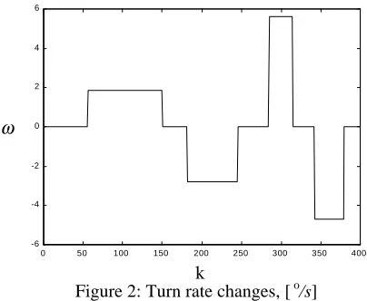
The scenario simulated here is very similar to those described in [4]. It includes few rectilinear stages and few CT maneuvers (Figs.1 and 2). Four consecutive 180

turns with rates

ω =

1.87, -2.8, 5.6, -4.68 [ o/s], are simulated, respectively for scans [56,150], [182, 245], [285, 314], [343,379].

1.5 2 2.5 3 3.5 4 4.5 5 5.5 6 x 104 2.5

3 3.5 4 4.5 5 5.5 6

x 104

X m, [ ]

Y m, [ ]

[image:5.595.307.515.161.321.2]

k=0

Figure 1: The test trajectory

The initial target position and velocities are

X

0

=

60[km],

Y

0

=

40[km],

X

0

= −

172

[m/s],

Y

0

=

246 [m/s] (i.e. aircraft speed 300 [m/s]). It is assumed that the sensor measures Cartesian coordinates

X and Y

instead the target range, bearing and range rate. It is also assumed that

σ

X

=

σ

Y

=

85

[m].

0 50 100 150 200 250 300 350 400

-6 -4 -2 0 2 4 6

ω

k

Figure 2: Turn rate changes, [ o/s]

5.3 Measures of performance

The Normalized estimation error squared (NEES), the mean error (ME), and the root mean-square error (RMSE) of each state component have been chosen as measures of performance. The ME and the RMSE of both estimated coordinates, as well as the ME and RMSE of both velocities have been respectively combined. The NEES of the AIMM algorithms is computed on the basis of the first four components from the augmented vector

[image:5.595.313.515.462.628.2]

(6)

5.4 Algorithms’ parameters

The algorithms are implemented with the set of parameters presented bellow:

• all algorithms use the next initial control parameter

ω

max

=

5 6

.

, [

o

/s];

• process noise standard deviations:

Algorithm

σ

_{v CV}_,

[m/s

2

]

σ

_{v CT}_,

[m/s

2

]

σ

_ω

[

o

/s]

FS AIMM

0

10

-2

VS

AIMM

0

10

-2

AGIMM

1.8

2.5

-• for the FS AIMM and VS AIMM:

Q

CV a

v CV

=

σ

,

2

,

Q

CT

diag

{

}

a

₌

0

0 σ

_ω2 ; Here, the AIMM algorithms maneuverability is achieved by the appropriately adjusted control parameter

ωi k

, , as well as by appropriately chosen value

σ

ω

2

(given in the above table). It provides minimal possible position and velocity RMSE .

• for the AGIMM:

Q

_CV

=

σ

_{v CV}, 2

,

Q

_CT

=

σ

_{v CT}, 2

. • fudge factor of the EKF using ACT:

φi

=

1

. • other AGIMM parameters:

δ

ωmin =23

ω

max

[o/s],

δ

_ωmax

=

ω

_max=5.6 [o/s];

05 .

0

1

=

t

,

t

2

=

0 92

.

;

• other VS AIMM parameters:

[

]

ω

i ,k ∈1 87 5 6. , . [

o_{/s], for}

_i

=

_{1 3}

_,

_;

• initial IMM mode probabilities:

[

]

µ

0

µ

0

µ

0

0 1 0 8

0 1

FS AIMM

₌

VS AIMM

₌

AGIMM

₌

.

';

• transition probabilities:

Pr

. . .

tr FS AIMM ₌



   



    0 6 0 3 0 1 0 1 0 8 0 1 0 1 0 3 0 6

,

Pr Pr

. . .

tr VS AIMM

tr AGIMM

= =



   



   

0 8 0 1 0 1

0 1 0 8 0 1 0 1 0 1 0 8

;

• initial error covariance matrices

P

T

FS AIMM VS AIMM

X X

Y Y

0 0

2 2

2

2 2

2

0

2

0

2

0

0 =

=













σ

_ω ,

where the sensor measurement errors are simulated for

σ

X

=

σ

Y

=

85

[

m

]

,

T

=

1

[

s

]

is the sampling interval. The respective matrix

P

0AGIMM of the VS AGIMM can be

obtained from the above matrix by excluding the last row and column from it.

5.5 Results

The measures of performance are computed upon the base of 100 independent Monte Carlo simulation runs. Respective plots are given in Figs.3-14. Their analysis leads to the next inferences:

1. All three investigated IMM algorithms show very good and very close performance. The established AIMM turn rate feedback provides significant algorithm’s self-adjustment abilities and maneuverability.

2. The ME plots (Figs. 3, 4) and the plots of the average turn rates (Figs. 11-13) confirm the better dynamics of both VS IMM algorithms compared to the FS IMM. The AGIMM algorithm is the most “mobile” algorithm due to its “artificial” abilities for instantaneous turn rate adjustment.

0 50 100 150 200 250 300 350 400

-60 -40 -20 0 20 40 60

VS AIMM

FS AIMM AGIMM

[image:6.595.60.293.152.271.2]

k

Figure 3: Position ME [m]

0 50 100 150 200 250 300 350 400

-50 -40 -30 -20 -10 0 10 20

AGIMM

FS AIMM VS AIMM

k

[image:6.595.55.519.344.778.2]

(7)

3. Both VS algorithm versions possess similar accuracy, slightly better than those provided by the FS AIMM algorithm (Figs.5,6).

4. Taking into account Figs. 1,2 and Figs.11-13 it may be stated that the continuous estimation in the VS AIMM algorithm provides the best turn rate estimation for the currently topical model.

5. The FS AIMM algorithm possesses the best overall consistency (Fig.14) due to the applied “natural” EKF mechanism for control parameter estimation.

0 50 100 150 200 250 300 350 400

35 40 45 50 55 60 65 70 75 80

AGIMM

k

VS AIMM

[image:7.595.324.514.64.212.2]

FS AIMM

Figure 5: Position RMSE [m]

0 50 100 150 200 250 300 350 400

10 15 20 25 30 35 40 45 50 55 60

k AGIMM

[image:7.595.79.282.214.752.2]

FS AIMM VS AIMM

Figure 6: Velocity RMSE [m/s]

0 50 100 150 200 250 300 350 400

0 1 2 3 4 5 6 7 8

FS AIMM

VS AIMM

k

Figure 7: RMSE of the overall estimate

∆

ω

k[

o

/s]

0 50 100 150 200 250 300 350 400 0.1

0.2 0.3 0.4 0.5 0.6 0.7 0.8

k µk

C

µk R

µk L

Fig. 8 FS AIMM average mode probabilities

0 50 100 150 200 250 300 350 400

0.1 0.2 0.3 0.4 0.5 0.6 0.7 0.8

µk

C µ_kL

µk R

[image:7.595.328.514.248.401.2]

k

Figure 9: VS AIMM average mode probabilities

0 50 100 150 200 250 300 350 400

0.1 0.2 0.3 0.4 0.5 0.6 0.7 0.8

µkC

µk R

µk L

k

Figure 10: AGIMM average mode probabilities

0 50 100 150 200 250 300 350 400

-15 -10 -5 0 5 10 15

k

ωk R

ωk L

[image:7.595.327.514.417.576.2]

ωk C

Figure 11: Average FS AIMM turn rates

ω

i k,

ω

i

ω

i k k, /

[image:7.595.329.515.598.780.2]

(8)

0 50 100 150 200 250 300 350 400 -6

-4 -2 0 2 4 6

ωk L

ωk C

ωk R

[image:8.595.80.270.64.217.2]

k

Figure 12: Average VS AIMM turn rates

ωi k

_, , [o/s]

0 50 100 150 200 250 300 350 400

-6 -4 -2 0 2 4 6

ωkL

ωk

C

ωk

R

[image:8.595.84.268.248.393.2]

k

Figure 13: Average AGIMM turn rates, [o/s]

0 50 100 150 200 250 300 350 400

0 5 10 15 20 25

AGIMM

VS AIMM

[image:8.595.80.267.428.576.2]

k FS AIMM

Figure 14: Normalized Estimation Error Squared

6 Conclusions

A new variable structure Augmented IMM technique is proposed in the paper. Fixed structure and variable structure AIMM algorithms using augmented constant velocity and augmented coordinated turn models are developed in the paper. The augmented coordinated turn model includes the difference between the unknown current turn rate and its value fixed in the IMM algorithm. As the simulation results show, this inclusion provides significant self-adjustment abilities to both proposed algorithms, resulting in very good overall accuracy and consistency. Compared to a particular VS adaptive grid IMM algorithm, both VS IMM algorithms show higher

mobility, while the FS AIMM algorithm possesses better consistency. The VS AIMM algorithm provides the best estimation of the turn rate.

References

[1] Bar-Shalom, Y., ed., Multitarget-Multisensor Tracking: Applications and Advances, Vol.2, Artech House, 1992.

[2] Bar-Shalom, Y., and X.R. Li, Estimation and Tracking Principles, Techniques and Software, Artech House, 1993.

[3] Blom H. A. P., Y. Bar-Shalom, The Interacting Multiple Model Algorithm for Systems with Markovian Switching Coefficients, IEEE Trans.on AC, Vol.33, No.8, pp.780-783, 1988.

[4] Jilkov, V., D. Angelova, and Tz. Semerdjiev, Mode-Set Adaptive IMM for Maneuvering Target Tracking, IEEE Trans. on AES, Vol.35, No.1, pp.343-349, 1997. [5] Li, X.R., Multiple-Model Estimation with Variable

Structure: Some Theoretical Considerations, In Proc. of 33rd IEEE Conf. Decision & Control, Orlando, FL, pp.1199-1204, 1994.

[6] Li, X. R., Hybrid Estimation Techniques. In Control and Dynamic Systems, C.T. Leondes, ed., Vol.76, pp.213-287, Academic Press, 1996.

[7] Li, X.R., Engineers' Guide to Variable-Structure Multiple-Model Estimation, in Y. Bar-Shalom and W.D.Blair, eds., Multitarget-Multisensor Tracking: Advances and Applications, Vol. 3, Artech House, 1999.

[8] Li, X.R., Y. Bar-Shalom, Design of an Interacting Multiple Model Algorithm for Air Traffic Control, IEEE Trans. on Automatic Control, Vol.1, No. 3, pp.186-194, 1993.

[9] Munir, A., D. Atherton, Maneuvring Target Tracking Using Different Turn Rate Models in the IMM Algorithm, in Proc. of the 34th Conf. on Decision & Control, New Orleans, 1995.

[10] Semerdjiev, E., L.Mihaylova, Adaptive IMM Algorithm for Manoeuvring Ship Tracking, In Proc. of the 1st Intern. Conf. on Multisource-Multisensor Information Fusion, Vol.2, pp.974-979, Las Vegas, USA, July 6-9, 1998.

[11] Semerdjiev, E., L. Mihaylova, L., and X. R. Li, An Adaptive IMM Filter for Aircrafts Tracking, In Proc. of the 2nd Intern. Conf. on Multisource-Multisensor Information Fusion, pp.770-776, Sunnyvale, CA, USA, 1999.

[12] Mihaylova, L., E.Semerdjiev, and X.R. Li, Detection and Localization of Faults in System Dynamics by IMM Estimator, In Proc. of the 2nd Intern. Conf. on Multisource-Multisensor Information Fusion, pp.937-943, 1999, Sunnyvale, USA.