Reference Dependence and Market Competition

Munich Personal RePEc Archive

Reference Dependence and Market

Competition

Zhou, Jidong

University College London

May 2008

Online at

https://mpra.ub.uni-muenchen.de/9370/

Reference Dependence and Market Competition

∗

Jidong Zhou

Department of Economics

University College London

First Version: October 2007. This Version: May 2008

Abstract

This paper studies the implications of consumer reference dependence in market competition. If consumers take some product (e.g., the first product they have con-sidered) as the reference point in evaluating others and exhibit loss aversion, then the more “prominent” firm whose product is taken as the reference point by more consumers will randomize its price over a high and a low one. All else equal, this firm will on average earn a larger market share and a higher profit than its rival. The welfare impact is that consumer reference dependence could harm firms and benefit consumers by intensifying price competition. Consumer reference dependence will also shapefirms’ advertising strategies and quality choices. If advertising increases product prominence, ex ante identical firms may differentiate their advertising intensities. If firms vary in their prominence, the less prominentfirm might supply a lower-quality product even if improving quality is costless.

Keywords: advertising, competition, loss aversion, product quality, reference depen-dence

JEL classification: D11, D43, L13, M37

1

Introduction

Economists have recently shown great interest in studying the market implications of hu-man behavioral biases (see, for example, Ellison (2006)). A branch of this literature investi-gates how consumers’ reference-dependent preferences (Kahneman and Tversky (1979,91)) influence thefirm’s behavior in the market. A mainfinding is that consumer loss aversion can cause price stickiness (Heidhues and K_˝oszegi (2007), for instance). Complementary to this view, this paper will present a model to argue that consumer loss aversion can also give rise to price variation in a competitive market and help explain sales in the market.

Our model is motivated by the fact that people often encounter and consider options sequentially, and lots of evidence has shown that the option which is considered (or tried)

∗_{I am indebted to Steffen Huck and Mark Armstrong for their guidance and many helpful discussions.}

first could be favored disproportionately even if there is little cost involved in moving to options considered later.1 One explanation, based on reference dependence, is that people tend to regard thefirst option as the reference point when they come to value later ones, and they display loss aversion in the sense later options’ relative disadvantages are weighed more than their relative advantages. Thus, all else equal, the early option may outperform later ones.2

Specifically, we consider a duopoly model with differentiated products where consumers consider or try products sequentially. We suppose that consumers take thefirst product as the reference point when they value the second one, and they exhibit loss aversion in both the price dimension and the product dimension: they are excessively averse to paying a price higher than the reference price or to having a product less well matched than the reference product. Another ingredient of our model is that one firm might be more “prominent” than the other in the sense that the prominent product is considered

first and so taken as the reference product by more consumers. The prominent product could be the default option, the product which is more heavily advertised, the product which is recommended or displayed more visibly in the store, and the product which enters the market earlier and consumersfirst hear of. The main question we investigate is how firms will strategically adjust their prices and product attributes to manipulate consumers’ reference points in a competitive environment, and what the impact of this strategic behavior on the market is.

Sections 2 and 3 investigate the pricing and welfare implications of consumer reference dependence. Section 2 considers the case where all consumers take the same product as the reference product. Such a relatively simple setting helps illustrate the key feature of our model: firms’ price choices have a direct bearing on consumers’ price sensitivity. If the referencefirm charges a lower price than its rival, loss aversion in the price dimension makes consumersmore price sensitive; if the reference firm charges a higher price, loss aversion in the product dimension makes the marginal consumer who must have a strong state for the reference productless price sensitive. Graphically, the reference firm’s demand curve has an inward kink at its rival’s price. In contrast, the other firm’s demand curve has an outward kink. With this new function for price, the reference firm has an incentive to randomize its price. It will either charge a lower price than its rival to earn a large market share or charge a higher price to focus on high-value consumers. But the other

firm will charge a medium price constantly. We further show that, all else equal, the

1_{For example, Madrian and Shea (2001) identify a default effect with employee savings plans. They}

find that participation in such schemes is significantly higher under automatic enrollment, and a substantial fraction of participants under automatic enrollment choose both the default contribution rate and fund allocation even though few employees hired before automatic enrollment picked this particular outcome. A similar default effect in automobile insurance purchases is documented by Johnson et al. (1993). Ho and Imai (2006) and Meredith and Salant (2007) observe that being listedfirst on the ballot paper can significantly increase a candidate’s vote share. See also relevant experimental evidence in, for example, Samuelson and Zeckhauser (1988) and Kahneman et al. (1991).

2_{The reference-dependent effect does not necessarily require that people possess the reference product}

reference product is on average more expensive and occupies a larger market share, and the referencefirm also earns a higher profit. Section 3 considers a more flexible setting which allows for heterogenous reference products among consumers. There the prominent

firm plays the same role as the referencefirm and similar results hold.

One implication of our price result is, if sellers in the market are not equally prominent, the more prominent one (for instance, the seller advertising more heavily or that having an advantageous location in a shopping area) may charge more volatile prices (for example, put its product on sales more frequently). This offers a new justification for the existence of sales in the market:3 _{sales can be used to manipulate consumers’ price sensitivity when}

a majority of consumers consider a certain productfirst in their market search process.4 The main welfarefindings are: (i) More severe loss aversion could intensify price com-petition, this harmingfirms and benefiting consumers. However, it usually leads to lower total welfare in our setting with inelastic demand. This is mainly because more severe loss aversion tends to enlarge the price difference between products and thus induce a worse matching of consumers along the personal taste dimension. (ii) Although the prominent product is on average more expensive, it may be better for consumers to consider itfirst, because doing so will prevent them from being over “addicted” to the low price at the expense of taste satisfaction.

Section 4 considers endogenous prominence and justifies asymmetric prominence as an equilibrium outcome of an extended game. We first show that a greater prominence difference betweenfirms can boosteachfirm’s profit. The intuition is, when afirm becomes relatively more prominent, it will rely more on those strong-taste consumers and so charge the high price more frequently, which will relax the price competition. Based on this result, we argue that iffirms sell their products through a platform, the platform has an incentive to make the two products unequally prominent; iffirms have an advertising competition and if advertising only increases product prominence, then ex ante identical firms may differentiate their advertising intensities.

Section 5 studies the case with asymmetric product qualities. We show that a relative increase of the prominentfirm’s product quality could benefit both firms. This is because letting consumers consider a higher quality productfirst can make them in aggregate less price sensitive and thus relax price competition. Therefore, if there is a quality choice stage prior to the price competition, the less prominent firm may have an incentive to supply a lower-quality product than its prominent rival even if it is costless to improve quality. This offers an alternative explanation for quality differentiation in the market.5

3_{Sales can also be explained as a result of intertemporal price discrimination (Sobel (1984), for instance)}

or price discrimination across captive and non-captive consumers (Varian (1980), for instance) in the single-product market, or as the loss-leader pricing strategy in the multi-single-product market (Lal and Matutes (1994)). See, for example, Hosken and Reiffen (2004) for a recent empirical study of sales.

4_{In particular, our price prediction is also consistent with the observation that the prices of national}

brands in supermarkets are often more volatile than the prices of private brands, if consumers tend to regard the national brand as the reference point. For example, Slade (1998) documents that the private-label prices of saltine crackers in U.S. are less volatile than major-manufacturer prices. Muller et al. (2006) provide similar evidence that the average number of price changes is significantly smaller for private label products than for national brands.

5_{In the conventional literature on vertical product differentiation (Shaked and Sutton (1982), for}

Related Literature:

Since the seminal work by Kahneman and Tversky (1979), it has been well established that people’s preferences are often influenced by some reference point and characterized by loss aversion.6 _{This behavioral regularity has been extensively applied to explain many}

economic anomalies such as the endowment effect, the status quo bias, and small-stake risk aversion (see, for example, Kahneman and Tversky (2000), and Della Vigna (2007)). However, relatively fewer articles investigate the firm’s response to consumer reference dependence. Most of the existing works study how a monopoly firm makes its dynamic pricing decision when consumers tend to regard the historical price as the reference price (see, for example, Fibich et al. (2007) and references cited therein).7 A main result is, if consumers display loss aversion, then thefirm should charge a constant price.8

Nevertheless, competition is important for investigating the market implications of consumer biases.9 Our work makes a step in this direction. A related recent paper is Heidhues and K˝oszegi (2007). Following K˝oszegi and Rabin (2006), they use consumers’ rational expectations of possible transaction results as the reference point. They then argue that loss aversion might give rise to “focal pricing” in the sense that firms may not adjust their prices even if their costs have changed andfirms with different costs may charge the same price. A simple argument can go as follows. Suppose that consumers expect to pay some fixed price before they enter the market. Then, due to loss aversion, eachfirm’s demand will becomemore price responsive if its actual price ishigherthan that expected fixed price, and so at that price the demand curve has an outward kink. This could drive all firms to actually charge that fixed price for a range of cost conditions.10 The main difference between their model and ours is that consumers in their model take the expectation as the reference point, so no individualfirm’sactual decision can influence it; while our reference point is some real product in the market, sofirms can manipulate it directly. This is the key reason why two models have different pricing predictions. Since the formation of reference points is usually context dependent, it is highly desirable to examine how different assumptions of reference points could lead to different market implications. In addition, we also investigate the impacts of consumer reference dependence on firms’ advertising and product quality choices.11

differentiate their qualities to soften price competition.

6_{Besides reference-dependent preferences and loss aversion, the other two elements of Kahneman and}

Tversky’s prospect theory are diminishing sensitivity (which implies risk aversion in the domain of gains and risk seeking in the domain of losses) and nonlinear decision weights (in the environment with uncertainty), but they are irrelevant in our model.

7_{Putler (1992) is an early theoretical attempt to introduce the reference-price effect into consumer}

demand theory. Gilboa and Schmeidler (2001) study the effect of satisficing behavior and adjustable aspiration levels on consumers’ dynamic choice, which bears some resemblance to the effect of reference-dependent preferences. However, neither paper studies how firms might respond to this non-standard consumer behavior.

8_{In contrast, if the effect of a gain is greater than a same-size loss, thefirm should price cyclically.} 9_{In addition, it is also desirable to take into account reference dependence in non-price product}

dimen-sions. Some empirical research (Hardie et al. (1993), for instance) suggests that loss aversion is even more severe in the product dimension than in the price dimension.

1 0_{See also their companion paper Heidhues and Koszegi (2005) which, among other results, shows a}

similar price-stickiness result in a static monopoly setting.

The reference-dependence effect in our model can be regarded as a particular kind of switching costs: moving from the reference product to the other involves psychological costs if the latter is relatively inferior in some aspects. But it is rather different from the traditional switching costs in both specifications and consequences (see, for example, Farrell and Klemperer (2007)). We will further discuss this difference in the end of Section 5.

Broadly, this paper also contributes to the emerging literature on behavioral industrial organization. For instance, Della Vigna and Malmendier (2004), Eliaz and Spiegler (2006), Gabaix and Laibson (2006), and Grubb (2006) study howfirms might take advantage of consumers’ limited abilities to forecast their future preferences. Armstrong and Chen (2007), Rubinstein (1993), and Spiegler (2006a,b) investigate how the heuristic decision making of consumers could induce firms to confuse consumers. Chen et al. (2005) and Shapiro (2006) examine the market implications of consumers’ limited memory.

2

Single Reference Product

2.1

Model

There are twofirms (1 and 2) in an industry, each supplying a distinct product at constant common unit cost, which we normalize to zero. They set pricesp1 and p2 simultaneously.

Consumers have diverse tastes for different products. We model this scenario via the Hotelling linear city. A consumer’s taste is represented by the parameter x which is distributed on the interval [0,1] according to a cumulative distribution function F(x) which is differentiable and has a positive density f(x). Firm 1 is exogenously located at the endpoint x= 0 and firm 2 is at the other endpoint x = 1. For a consumer at x, the match utility of product 1 isv−x, and that of product 2 isv−(1−x), wherevis the gross utility of the product and is assumed to be sufficiently large such that the whole market is covered in equilibrium.12 _{Consumers have unit demand for one product, and the number}

of consumers is normalized to one.

We introduce consumer reference dependence by considering a sequential-consideration scenario: consumers consider or try products one by one, and a product’s price and match utility are discovered when it is considered or tried. We assume that consumers will take the first product they consider as the reference point. When they come to the second one, they will value its relative advantage (lower price or higher match utility) in the standard way, while they will over weigh its relative disadvantage (higher price or lower match utility) in the spirit of loss aversion.13 _{We also assume that consumers do not}

include, for example, Compte and Jehiel (2003) (prior offers as reference points in sequential bargaining), Eliaz and Spiegler (2007) (the default alternative as the reference point in forming consideration sets), Hart and Moore (2007) (contracts as reference points inex posttrading relationship), and Rosenkranz and Schmitz (2007) (reserve prices in auctions as reference points in deciding on bidding strategies).

1 2_{Alternatively, we can assume that a product’s match utility is a random draw from some common}

distribution and its realization is independent across consumers and products. Our following analysis still applies to this setting by modifying notation slightly.

1 3_{In our model, the reference point is an individual product. An alternative specification of the reference}

intentionally choose the order in which they consider products, and they may just follow some natural presentation order of products or be guided byfirms’ marketing activities. (See a discussion about more sophisticated consumers in Section 3.) In this section, for simplicity we further suppose that all consumers will consider product 1 first (which is the default option, for instance), and we call it the reference product. (We will treat a moreflexible setting in Section 3.)14

One point deserves mention before proceeding. Although sequential consideration is a reasonable scenario to think about reference dependence, our model is actually not restricted to this interpretation. What we need is that consumers somehow take some product in the market as the reference point when they evaluate others. The details on why some product becomes the reference point is not crucial to most of our following analysis.

Consumer preferences are specified as follows. Given the prices p1 and p2, a consumer

atxvalues product 1, the reference product, in the standard way:

v−x−p1;

her valuation of product 2 is

v₋(1₋x)₋p2−(λ−1) max{0, p2−p1}−(λ−1) max{0,1−2x},

where the first three terms represent the standard intrinsic surplus of product 2 and the other two terms capture the potential reference-dependent “loss utility” in each dimension.

λ >1is the loss-aversion parameter and measures the strength of the reference-dependence effect.15 _{If λ = 1, we return to the orthodox Hotelling model. An implicit assumption}

here is that the reference-dependent “loss utility” occurs separately in the price dimension and the product dimension. It is psychologically reasonable and has been well supported in the literature of prospect theory (see, for example, Tversky and Kahneman (1991)). For simplicity, we have assumed the same degree of loss aversion in both dimensions. Considering asymmetric degrees of loss aversion in the two dimensions will not affect most of our main results qualitatively.16

To highlight how reference dependence could benefit the reference product, we first focus on the case with a symmetric distribution of consumers (i.e.,F(1₋x) = 1₋F(x)).

to that case qualitatively. However, the assumption that the reference point is from the market rather from outside (for example, some “ideal” product in a consumer’s mind before she enters the market) is important.

1 4_{Our one-shot model may be more suitable for infrequently purchased products or for frequently}

pur-chased products but with poor-memory consumers. Otherwise, the reference point might also be influenced by the historical purchase.

1 5_{The strength of the reference-dependence effect could be affected by the time lag between considering}

options. If the time lag is too long, people may have forgotten thefirst option when they value the second one; if it is too short, people may have not adapted themselves to thefirst option when the second one comes. Hence, the effect might be most pronounced when the time lag is appropriate. Presumably, the effect would be also more pronounced if consumers encounter alternative options somehow unexpectedly. If people have been expecting to consider other options when they encounter thefirst one, they may not attach to it too much and so the reference dependence effect might be weak.

1 6_{Our welfare results could be affected if the degrees of loss aversion in the two dimensions differ}

That is, there is no systematic quality difference between the two products. (We will discuss the impact of asymmetric qualities in Section 5.) We also assume away any possible explicit costs involved in moving from one product to the other. Introducing such costs will bringfirm 1 with an extra advantage.

Now we are ready to derive each firm’s demand function. We claim that if firm 1 chargesp1< p2, its demand function is

q1(p1 < p2) =F

µ

1 2 +

λ

2(p2−p1)

¶

. (1)

This is because all consumers with x ≤ 1

2 will definitely buy product 1, and those with

x > 1₂ will buy product 1 only if the gain from product 2’s higher match utility is less than the loss (including the psychological part) from its higher price, i.e., only if2x₋1< λ(p2−p1), which leads to

x < 1

2 +

λ

2(p2−p1).

It is ready to see that consumers are now more price sensitive than in the orthodox model (which applies whenλ= 1). This is because the attractiveness of firm 1’s lower price has been amplified by consumers’ loss aversion in the price dimension.

When firm 1 charges p1 > p2, all consumers with x > 1₂ will buy product 2, and

those withx < 1₂ will choose product 1 only if the loss (including the psychological part) from product 2’s lower match utility exceeds the gain from its lower price, i.e., only if

λ(1−2x) > p1 −p2. Now those consumers with x < 1₂ become less price sensitive,

because the unattractiveness offirm 1’s higher price has appeared less important relative to the unattractiveness of product 2’s lower match utility. The corresponding demand function is

q1(p1 > p2) =F

µ

1 2+

1

2λ(p2−p1)

¶

. (2)

(1) and (2) imply that, aroundp2,firm 1’s demand is more price responsive atp1 < p2

than atp1 > p2, and hence the demand curve has an inward kink at p1 =p2 (see Figure

1 below which illustrates the case with uniformx).

Firm 2’s demand is q2 = 1−q1. Explicitly, using the symmetry of distribution, we

have

q2(p2 > p1) =F

µ

1 2+

λ

2(p1−p2)

¶

; q2(p2 < p1) =F

µ

1 2 +

1

2λ(p1−p2)

¶

. (3)

When p2 > p1, the unattractiveness of firm 2’s higher price will be amplified by loss

aversion since consumers regardp1as the reference price. Whenp2 < p1, the attractiveness

of its lower price to the marginal consumer atx < 1₂ will be reduced by her extra aversion to product 2’s lower match utility. Clearly, around p1, firm 2’s demand is more price

responsive at p2 > p1 than at p2 < p1, which implies that q2 has an outward kink at

HH HH

HH_HH

A A A A A A A q1

p1

p2

1/2 _A

A A

A A

A AA H

H H H H H H H q2

p2

p1

1/2

Figure 1: An Illustration of Demand Curves

In sum, compared to the orthodox case, consumers will become more (less) price sensitive if the reference product is cheaper (more expensive) than the other. Moreover, consumer reference dependence benefits the referencefirm but harms the other in the sense that, at any pair of pricesp1 6=p2,q1 increases but q2 decreases relative to the orthodox

case.

Two additional properties of the demand function deserve mention. First, q1 > q2 if

and only ifp1< p2. In effect, reference dependence does not affect eachfirm’s demanded

quantity if they charge the same price. However, it still affects the price sensitivity at that point. Second, at anyfixed price pair p1 6=p2, bothfirms’ demand curves have the same

slope given q2 = 1−q1.17 In the following, we denote by πi(p1, p2) =pi·qi(p1, p2) the

profit function of firmi.

2.2

Equilibrium

Now we derive the Nash equilibrium of the price competition. First of all, both firms charging the same price is not an equilibrium. Given a positive price offirm 2, firm 1’s demand has an inward kink at this price, which means that its profit function has a local minimum at this point. Hence, charging the same price will never befirm 1’s best response. Second, there is no asymmetric pure-strategy equilibrium either. Supposep1 6=p2 were an

equilibrium. Since bothfirms face the same demand slope at this hypothetical equilibrium point, in equilibrium the firm charging the higher price should have a higher demand.18

But that is impossible in our symmetric environment. We formalize the above argument in the following proposition. All omitted proofs are presented in the Appendix.

Proposition 1 Given a symmetric distribution of consumers, the price competition has no pure-strategy Nash equilibrium.

We will then show that, under regularity conditions, the game has a mixed-strategy equilibrium in whichfirm 1 charges a low pricepL

1 with probabilityμ∈(0,1) and a high

1 7_{This property does not depend on the assumption of a symmetric distribution of consumers.}

1 8_{This is because, in a hypothetical asymmetric equilibrium, each firm’s demand function is smooth}

price pH

1 with probability 1−μ, and firm 2 charges a medium price p2 for sure. Given

firm 1’s mixed pricing strategy, let

qe₂(p;μ, pL₁, pH₁ ) =μ·q2(pL1, p) + (1−μ)·q2(pH1 , p) (4)

be firm 2’s expected demand function. It has two outward kinks at pL₁ and pH₁ which divide it into three segments (see Figure 2 below). The regularity conditions are:

Assumption 1 (i) f(x) is logconcave;19 _{(ii) for μ ∈ (0,1) and 0 < p}L

1 < pH1 , each

segment of q₂e is regular such that the corresponding part of firm 2’s profit function is quasi-concave.20

Notice that the uniform distribution (F(x) =x) satisfies Assumption 1 since then each segment ofqe₂ is linear.

Proposition 2 Given a symmetric distribution of consumers and Assumption 1,21 there exists a mixed-strategy equilibrium as specified in the above where the quadruplet(μ, pL

1, pH1 , p2)

satisfies the following conditions: (i) p2 = arg maxpp·qe2(p;μ, pH1 , pL1);

(ii) pL₁ = arg maxp≤p2p·q1(p, p2), and pH1 = arg maxp≥p2p·q1(p, p2);

(iii) π1(pL1, p2) =π1(pH1 , p2).

Conditions (i) and (ii) define each firm’s best response given its rival’s strategy, and condition (iii) means thatfirm 1 is indifferent between charging the low and the high price. A potential complication is, ifλis sufficiently large,firm 1 may occupy the whole market when it charges the low price pL

1. As we discuss in Appendix A.2, such an equilibrium

with a corner solution can actually occur. However, in the main text of this paper (except in Section 5), we focus on the interior-solution equilibrium in which no firm captures all consumers (which requires relatively smallλ).

We illustrate the equilibrium in Figure 2 below which is based on the uniform-distribution case, whereπi isfirmi’s iso-profit curve. The intuition of this mixed-strategy equilibrium

is as follows. Givenfirm 2’s price,firm 1 can either charge a lower price to make consumers more price sensitive and then earn a large market share, or charge a higher price to exploit those consumers who have a strong taste for its product and will thus become less price sensitive due to loss aversion in the taste dimension.22 _{Although these two strategies are}

1 9_{The logconcavity condition is satisfied by many well-known (truncated if necessary) distributions. See,}

for example, Bagnoli and Bergstrom (2005) for a detailed discussion.

2 0_{Since logconcavef implies logconcaveF,firm 1’s demand in each side of its kink is logconcave such}

that the corresponding part of its profit function is logconcave (so quasi-concave). (Remember that firm 1’s whole profit function will never be quasi-concave.) However, a weighted average of two logconcave functions may fail to be logconcave. In our case, thoughq2(pi1, p)is logconcave under (i),q2e(p)defined in

(4) may not be. That is why we need (ii). But one can show that (i) implies (ii) ifλis close to one or if

f0₍₀₎

f(0) < 4 1+λpH

1 . (The latter condition actually implies concave profit function offirm 2.)

2 1_{If Assumption 1 fails to be satisfied, we may have other types of mixed-strategy equilibrium. But note}

that the general existence of equilibrium is no problem according to the Glicksberg Theorem, since each firm’s profit function is continuous and we can restrict eachfirm’s feasible prices to a compact interval.

2 2

This argument does not apply to firm 2. Givenfixedp1, iffirm 2 charges a higher price, consumers

will become more price sensitive, which will drivefirm 2 to lower its price; iffirm 2 charges a lower price thanp1, the marginal consumer who has a strong taste for product 1 will become less price sensitive, which

equally profitable in equilibrium, firm 1 will not adopt either strategy predictably. Oth-erwise,firm 2 would either be attempted to charge a low price to steal business when pH₁

applies, or be forced to match pL

1 to protect its own market share. Either situation will

lower firm 1’s profit, so firm 1 has an incentive to randomize its price and keep firm 2 guessing.

Figure 2: An Illustration of the Equilibrium

• The robustness of equilibrium. Readers may wonder whether there are other types of mixed-strategy equilibrium in our model. A sufficient condition for the uniqueness of our equilibrium is, on top of Assumption 1, for any possible mixed pricing strategy of

firm 1, firm 2’s expected profit function will be globally quasi-concave. We do not have primitive conditions for this, but it is satisfied at least by the uniform distribution as we will show in Section 3.

Our equilibrium is robust to heterogenous reference points among consumers. For example, when product 1 is more heavily advertised than product 2, more than half consumers may notice and consider product 1first and others may notice product 2 first. We will investigate such a general setting in Section 3, and there we will show that a similar equilibrium exists provided that the two products are not equally noticeable. It is also not difficult to extend our model to the case with more than twofirms, if consumers still take some product as the reference point in evaluating others.23 No fundamental changes will take place since howfirms’ price choices affect the price sensitivity of consumers remains unchanged.

2 3

Another issue is about the assumption of symmetric distributions. From the proofs of Propositions 1 and 2, we can see that this assumption can be replaced by a weaker condition: F(1₂) = 1₂. Beyond this, will our mixed-strategy equilibrium still persist? The following proposition tells us that, given the degree of loss aversion, our equilibrium continues to hold provided that the distribution is not too skewed to either endpoint.

Proposition 3 Given Assumption 1,

(i) for fixed λ, there exists ε > 0 such that, when ¯¯F(1₂)₋1₂¯¯ < ε, there is no pure-strategy equilibrium, and a similar mixed-pure-strategy equilibrium as before exists;

(ii) for fixed¯¯F(1₂)₋1₂¯¯>0, there exists λ∗ >1 such that, when λ < λ∗, there is only a pure-strategy equilibrium with p1> p2 if F(1₂)> 1₂ and p1< p2 if F(1₂)< 1₂.

Part (ii) of this proposition means that, given an asymmetric distribution, if the degree of loss aversion is sufficiently low, pure-strategy equilibrium will emerge. We will further illustrate this result in Section 5 when we discuss asymmetric product qualities (which is a special case of asymmetric distributions).

• The benefit of selling the reference product. We then investigate whether the reference firm enjoys an advantage over its rival merely due to consumer reference dependence. As we can see from the demand function, if the reference firm charges a higher price than its rival, the shrink of its market share will be mitigated by consumers’ loss aversion in the product dimension; and if it charges a lower price, the expansion of its market share will be amplified by consumers’ loss aversion in the price dimension. In either case, consumer reference dependence favors the reference firm. Thus, we should expect that the reference firm will earn more the other. In addition, we will also compare the twofirms’ average prices and market shares, of which the results are not easy to predict in advance given the mixed-strategy equilibrium.

Proposition 4 Given a symmetric distribution of consumers and Assumption 1, in the mixed-strategy equilibrium we have identified,

(i) firm 1 charges the high price more frequently (μ < 1₂) and product 1 is on average more expensive than product 2 (pe

1 =μpL1 + (1−μ)pH1 > p2);

(ii) on average firm 1 occupies a (weakly) larger market share than firm 2 (q₂e ≤ 1 2),

and they share the market equally if and only if the distribution is uniform; (iii) firm 1 earns strictly higher profit thanfirm 2.

There are two other questions deserving investigation. First, how will price and welfare vary with the degree of loss aversion? Second, givenfirms’ equilibrium pricing strategies, if consumers realize their own biases and can choose the consideration order freely, is it really in their own interests to consider the reference productfirst? Due to the tractability issue, we discuss them in the uniform-distribution case in next section.

3

Heterogeneous Reference Products

product, while 1_{2 −}θ of consumers will take product 2 as the reference product. Without loss of generality, let θ ∈ [0,1₂]. When θ > 0, we say product 1 is more “prominent” than product 2, and θ indicates the prominence difference between the two products. This flexible setting will allow us to discuss endogenous prominence through advertising competition in Section 4.

3.1

The general case

Each firm now has two demand sources: those consumers regarding its product as a reference point and those regarding its rival’s product as a reference point. Whenfirm 1 chargesp1< p2, its demand function becomes

q1(p1 < p2) = (

1 2 +θ)F

µ

1 2+

λ

2(p2−p1)

¶

+ (1 2−θ)F

µ

1 2 +

1

2λ(p2−p1)

¶

.

The first part is the same as before, and the second part is because, among consumers who regard product 2 as the reference product, the marginal consumer is now at x > 1₂

and she will become less price sensitive due to her extra aversion to the less well matched product 1. Similarly,

q1(p1 > p2) = (

1 2 +θ)F

µ

1 2+

1

2λ(p2−p1)

¶

+ (1 2−θ)F

µ

1 2+

λ

2(p2−p1)

¶

.

Forθ_∈(0,1₂), we have

lim

p1→p−₂

q0

1(p1 < p2) =−

1 2f(

1 2)

∙

(1

2+θ)λ+ ( 1 2−θ)

1

λ

¸

< lim

p1→p+₂

q0

1(p1> p2) =−

1 2f(

1 2)

∙

(1

2−θ)λ+ ( 1 2+θ)

1

λ

¸

,

which means that q1 has an inward kink at p1 = p2. Firm 2’s demand function can

be treated similarly and it has an outward kink at p2 = p1. Therefore, compared to

the single-reference-product case, we should not expect any qualitative changes to take place. The counterparts of Propositions 1—3 can be proved similarly but with heavier notation. Although the counterpart of Proposition 4 has not been established completely, we conjecture it would hold. We will verify it in the uniform-distribution case below, and we can also verify it whenλis close to one.24

2 4_{Whenλ= 1 +εandεtends to zero, equilibrium prices can be approximated as}

pL1 ≈ p

∙

1−θε+ µ

3θ2−1−θ 2 −A

¶ ε2

¸ ,

pH1 ≈ p

∙

1 +θε+ µ

3θ2−1 +₂θ−A ¶

ε2 ¸

,

p2 ≈ p

∙

1 + (2θ2−1₂)ε2 ¸

, μ≈ 1₂−(θ 2+

A 2θ)ε,

where p = 1/f(1

2) is the equilibrium price in the standard Hotelling model and A =

θ2

p3

16 f00( 1 2). The

A notable exception is θ= 0(in which case the two products are equally prominent). In this symmetric case, the demand functions are smooth and we have a symmetric pure-strategy equilibrium with

p∗ = 2

(λ+ 1/λ)f(1/2).

Compared to the standard Hotelling model where λ = 1, loss aversion leads to lower equilibrium price sinceλ+1_λ >2. However, any extent of prominence difference between the twofirms will overturn this equilibrium.

3.2

The uniform-distribution case

In the following, we will proceed our analysis in the uniform-distribution case with asym-metric prominence (i.e., θ > 0). One justification for asymmetric prominence will be provided in Section 4 where we consider endogenous prominence through advertising com-petition.

Wefirst introduce two pieces of notation:

h= (1

2 +θ)λ+ ( 1 2−θ)

1

λ, l= (

1

2−θ)λ+ ( 1 2+θ)

1

λ.

Clearly,h > lwhen θ >0. Then the two firms’ demand functions can be written as

q1 =

1 2 +

i

2(p2−p1), q2= 1 2 +

i

2(p1−p2),

wherei=h ifp1 < p2 and i=l ifp1 > p2. So the demand is more price responsive when

the prominent product is relatively cheaper. When firm 1 uses the mixed strategy as in Section 2,firm 2’s expected demand function is

q₂e(p2) =

1 2 +

μh

2 (p

L

1 −p2) +

(1₋μ)l

2 (p

H

1 −p2), (5)

forp2∈[pL1, pH1 ].

In this uniform setting, the following condition guarantees the mixed-strategy equilib-rium with an interior solution:

1< r=

r

h

l <3. (6)

In particular, whenθ= 1₂, we haveh=λand l= 1_λ, so (6) requires λ <3. For smaller θ, (6) is easier to hold. For example, whenθ tends to zero,h andl will coincide, and so (6) is always true.

Wefirst derive equilibrium. (Note that, in the uniform setup, all following necessarily conditions are also sufficient.) Given p2,firm 1’s best responses imply

pL₁ = 1 2h +

p2

2 ; p

H 1 =

1 2l +

p2

2.

And the indifference condition requires

pL₁

∙

1 2 +

h

2(p2−p

L 1)

¸

=pH₁

∙

1 2 +

l

2(p2−p

H 1 )

¸

From them, we solve

pL₁ = 1 2 ∙ 1 h + 1 √ hl ¸

= 1 +r 2h ,

pH₁ = 1 2 ∙ 1 l + 1 √ hl ¸

= r(1 +r) 2h ,

p2 =

1

√ hl =

r h.

With the expected demand function in (5),firm 2’s best response implies

2 [μh+ (1₋μ)l]p2 = 1 +μhpL1 + (1−μ)lpH1 , (7)

from which we get

μ= 1 1 +r.

It is ready to see that pL₁ < p2 < pH1 and μ ∈ (0,12). For this solution to be a real

equilibrium, we further need that no firm captures all consumers. Simple calculation shows thatfirm 1’s demands are

qL₁ = 1 +r 4 , q

H 1 =

1 +r

4r

when it charges pL₁ and pH₁ , respectively. So (6) indeed guarantees an interior-solution equilibrium.

Moreover, this is the unique equilibrium. Since firm 2’s demand function is strictly concave for any fixed p1 in this uniform setting, its expected demand function is also

strictly concave for any mixed pricing strategy of firm 1. Firm 2 will therefore never randomize its price. On the other hand, for any fixed p2, firm 1’s demand function is

linear in each side of its kink, so it is impossible for firm 1 to have more than two best replies.

We then study the properties of equilibrium. Define

4L=p2−pL1 =

r−1

2h ; 4H =p

H

1 −p2 = r(r−1)

2h .

Then

4H

4L

=r >1, (8)

which means that, relative tofirm 2’s price,pH₁ deviates more thanpL₁. On the other hand,

firm 1 charges the high price pH₁ more frequently since μ < 1₂. These two observations imply that product 1 is on average more expensive than product 2:

pe₁ = 1 +r

2

2h > p2 = r h.

One can check thatfirm 1’s expected demand is just 1₂. That is, on average bothfirms share the market equally thoughfirm 1 is more prominent.25 _{Butfirm 1 earns more than} firm 2:

π1=

1 8 ∙ 1 √ h + 1 √ l ¸2

= (1 +r)

2

8h > π2= p2

2 =

r

2h. (9)

2 5

Thus, similar results as in Proposition 4 have been established in this heterogenous-reference-product setting with the uniform distribution.

We now answer those two questions proposed in the end of Section 2.

• Which product should consumers consider first? In our model, the order in which consumers consider product is specified exogenously or determined by firms’ marketing activities such as advertising. We have not yet consider the question that, if consumers realize their own behavioral biases and can choose their own consideration orders freely, how they will behave given thatfirms adopt the above equilibrium pricing strategies and they are distinguishable in the market.

We first set the welfare criterion. Throughout this paper, we take the view that the psychological “loss utility” only occurs in the decision process, and it affects the ultimate welfare status of consumers only through influencing their choices. Hence, we use the orthodox welfare measurement.26 Also remember that consumers do not know a product’s match utility until they consider it, so consumers are ex ante identical. Since pe₁ > p2,

people may conjecture that those considering product 2first would obtain higher surplus. This conjecture, however, isnot true.

Define

xL=

1 2 +

λ

24L; xH = 1 2 −

1

2λ4H. (10)

For a consumer considering product 1first, if its price ispi

1, she will buy product 1 if and

only if her location is less thanxi, so her expected surplus is v−αi, where

αi =

Z xi

0

(x+pi₁)dx+

Z 1 xi

(1₋x+p2)dx

is the sum of expected taste loss and expected payment. Thus, given firms’ strategies, the expected surplus of a consumer who considers product 1first isv₋μαL−(1−μ)αH.

Similarly, define

yL=

1 2 +

1

2λ4L; yH=

1 2 −

λ

24H. (11)

Then, the expected surplus of a consumer who considers product 2first isv₋μβ_L−(1₋

μ)β_H, where

β_i=

Z yi

0

(x+pi₁)dx+

Z 1

yi

(1−x+p2)dx.

Therefore, considering product 1first is better if

μαL+ (1−μ)αH< μβL+ (1−μ)βH. (12)

One can verify

αL−βL=

Z xL

yL

(2x−1)dx

| {z }

Increase of Taste Loss −

Z xL

yL

4Ldx

| {z }

Saving of Payment

= M 4 4

2 L>0,

2 6_{Even if we add the “loss utility” to welfare calculation, our following result still holds ifλis relatively}

where M = (λ₋1/λ) (λ+ 1/λ₋2) > 0. This means that, when firm 1 is charging the low price, considering its product first is actually worse than considering product 2

first. Two conflicting forces work here. On the one hand, if a consumer considers the cheaper productfirst, she will become excessively averse to paying a higher price due to loss aversion, and so she will be more likely to buy product 1 (i.e., xL > yL), which of

course can save expected payment. On the other hand, relative to the socially optimal situation in which consumers should buy the most matched product regardless of the price difference, xL > yL > 1₂ implies that considering the cheaper product 1 first will result

in more severe product-choice distortion and so involve a greater expected taste loss. It turns out that the latter negative effect dominates in our setting. Similarly, we have

αH−βH=

Z xH

yH

(2x₋1 +4H)dx=−

M

4 4

2 H <0.

That is, when firm 1 is charging the high price, considering its product first is actually better.

Now (12) becomes μ42_L<(1−μ)42_H, which, according to (8), is equivalent to

μ

1−μ < r

2_.

But this inequality must be true sinceμ < 1₂ and r >1.

Therefore, in the uniform-distribution setting with the orthodox welfare criterion, con-sidering the more prominent product 1first will yield higher expected consumer surplus. The reason is that considering the more expensive product first will prevent consumers from being over “addicted” to the low price at the expense of taste satisfaction.27,28

• The impact of loss aversion. We now turn to examine how price and welfare vary with the degree of loss aversion. We will show that, when the prominence difference between the two firms is relatively small, more severe loss aversion will intensify price competition, harmfirms and benefit consumers (which is consistent with the observation at θ = 0); when the prominence difference is relatively large, more severe loss aversion will tend to increase industry profit and harm consumers. In either case, more severe loss aversion leads to lower total welfare in our inelastic-demand setting.

Wefirst present some useful observations (remember r=

q

h l):

h l hl r

λ + ? + +

2 7_{We conjecture that this result would even hold for a general distribution, which can be verified at least}

in the limit case withλclose to one. However, if the extent of loss aversion in the price dimension is rather weak, then the result could be reversed. In particular, if there is no loss aversion in the price dimension, thenM = (1−1/λ)(1 + 1/λ−1)<0and so considering product 2first is better.

2 8_{One implication of our result is that, if consumers are sophisticated and they are able to choose their}

consideration order freely, our game withex ante symmetricfirms has three equilibria. In the symmetric pure-strategy equilibrium (withθ= 0), expecting both firms are charging the same price, consumers will consider products in a random order, which will further sustain the symmetric equilibrium. In the other two asymmetric equilibria (withθ= 1

2 and− 1

2, respectively), expecting onefirm is charging a random but

In this table, “+” means the variable in the row increases with the parameter in the column, and “?” means a possible non-monotonic relationship.29 (Note that, whenθ= 1₂,

hl= 1is independent ofλ. This caveat applies to all following analysis.)

Price. It is ready to see that bothp2= 1/

√

hl andpL

1 = 2h1 + p2

2 fall withλ. ButpH1

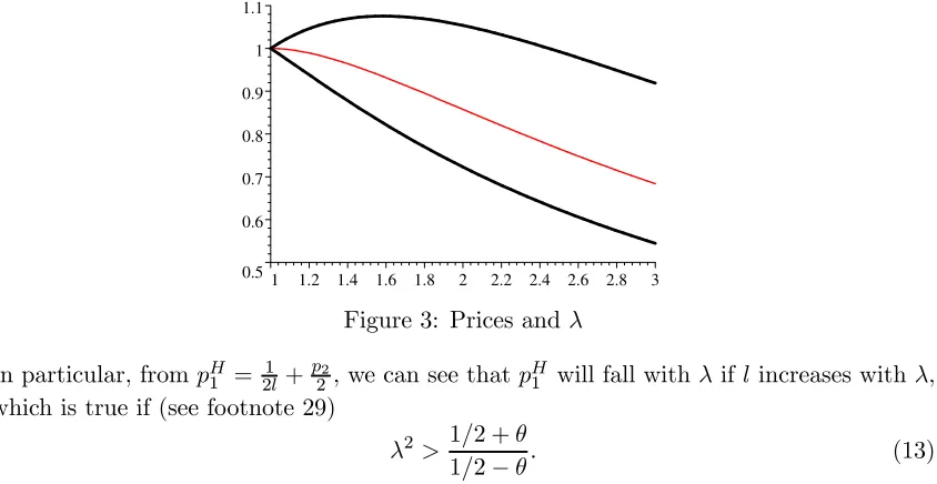
may vary withλnon-monotonically. Figure 3 below is a numerical example withθ= 0.3 where the thin line isp2.

0.5 0.6 0.7 0.8 0.9 1 1.1

1 1.2 1.4 1.6 1.8 2 2.2 2.4 2.6 2.8 3

Figure 3: Prices andλ

In particular, frompH₁ = _2l1 +p2₂, we can see that pH₁ will fall withλifl increases withλ, which is true if (see footnote 29)

λ2 > 1/2 +θ

1/2₋θ. (13)

This condition is easier to hold for higher λand lower θ. For example, when θ tends to zero, it is always true; whenθtends to 1₂, it fails for sure.30 _{Roughly speaking, for smaller} θ, firm 1’s profit from exploiting those strong-taste consumers by charging a high price will go down since now fewer of them will visitfirm 1first.

Profit. It is clear that π2 =p2/2 decreases with λ. But π1 could vary with λ

non-monotonically.31 In particular, sinceπ1= 1₈(h−1/2+l−1/2)2(see (9)), a sufficient condition

forπ1 to be decreasing withλis also (13) givenhincreases withλ. Therefore, it is possible

(at least under (13)) that more severe loss aversion will intensify competition and harm bothfirms.32

Consumer surplus and welfare. Remember that our welfare measurement does not include the psychological “loss utility”. LetW be total welfare andW =v₋T, where

T = 1 4

£

1 +μAL42L+ (1−μ)AH42H

¤

(withAL=h(λ+ 1/λ)−1andAH=l(λ+ 1/λ)−1) is the overall taste loss. Notice that,

if both firms charge the same price, then each consumer will buy the product she most

2 9

It is ready to show _∂λ∂l = 1₂ −θ−(1₂ +θ)λ−2. Thus,lincreases with λif and only ifλ2 > 1₁/_/2+₂₋θ_θ for θ <1

2.

3 0_Forθ=1

2,p2 is a constant, and sop

H

1 increases withλ.

3 1_{One can show that} ∂π1

∂λ has the sign of θ(r3

−1) 2 (1 +λ−

2₎₋r3

+1 4 (1−λ−

2_{). Thus, whenθtends to zero,}

∂π1

∂λ <0; whenθtends to

1 2,

∂π1

∂λ >0; and for intermediateθ,π1 could be non-monotonic withλ.

3 2_{However, it is also possible that more severe loss aversion will boost industry profit. This will happen}

at least whenθis close to 1

2, because atθ= 1

likes, which is socially optimal and leads to the minimum taste loss 1₄. When consumers exhibit reference dependence and θ > 0, there exists price difference between products, which will cause distortion in product choice. Specifically, when firm 1 charges pi

1 and

firm 2 chargesp2, the efficiency loss is

(1

2 +θ)(xi− 1 2)

2_{+ (}1

2 −θ)(yi− 1 2)

2 ₌ 1

4Ai4

2 i

wherexiandyihave been defined in (10) and (11). Consumer surplus isV =v−T−π1−π2.

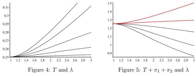
We consider the simple case with θ = 1₂ first. In this case, one can check 4T −1 = (λ−1)2/4λwhich goes up withλ, and so more severe loss aversion is detrimental to total welfare (and consumer surplus in the light of footnote 32). This welfare result is mainly driven by the fact that4i increases with λand larger price gaps imply greater

product-choice distortion and so lower efficiency. For θ < 1₂, numerical simulations suggest that

W still decreases with λ(see Figure 4 below where from the bottom to the top θ ranges from0.1 to0.5), but how V varies withλ depends onθ.33 Figure 5 below indicates that more severe loss aversion will be beneficial to consumers themselves when θ is relatively low. This is because, whenθis lower, it is more likely that higherλwill decrease all prices (see (13)).

0.25 0.26 0.27 0.28 0.29 0.3 0.31

1 1.2 1.4 1.6 1.8 2 2.2 2.4 2.6 2.8 3

Figure 4: T and λ

0.9 1 1.1 1.2 1.3 1.4 1.5

1 1.2 1.4 1.6 1.8 2 2.2 2.4 2.6 2.8 3

Figure 5: T+π1+π2 and λ

Discussion:

Now we discuss how asymmetric degrees of loss aversion in the two dimensions will affect our results. The influence can be seen from two extreme cases. (i) If loss aversion occurs only in the price dimension, all analysis applies if we useh= (1₂+θ)λ+ (1₂₋θ)and

l= (1₂ −θ)λ+ (₂1 +θ). Clearly, bothh and l increases with λ. One can verify that more severe loss aversion will then always intensify price competition such that all prices and profits decrease withλand consumer surplus increases withλ. So loss aversion in the price dimension is pro-competitive. (ii) If loss aversion occurs only in the taste dimension, all analysis also applies as long as we useh= (1₂+θ) + (1₂₋θ)/λandl= (1₂₋θ) + (1₂+θ)/λ. Now both h and l decreases with λ. It is not difficult to check that more severe loss version will now always soften price competition such that all prices and profits increase with λ and consumer surplus decreases with λ. So loss aversion in the taste dimension is anti-competitive. In either case, total welfare in our inelastic-demand setting still goes

3 3

down withλ. Our model with symmetric degrees of loss aversion is just a combination of these two extreme cases.

4

Endogenous Prominence: Platform and Advertising

Com-petition

In this section, we discuss two possible ways to endogenize prominence. One story is to consider a platform (for example, a supermarket) on which firms sell products. Suppose

firms can set product prices by themselves and the platform can charge each of them a fee proportional to their profit. Then does the platform have an incentive to manipulate consumers’ consideration order through adjusting the relative prominence among products (for example, displaying some product more visibly or recommending some product to consumers)? The other story is to consider advertising competition. For example, a consumer might first notice and then consider the product whose adverts first come to her attention, and then the more heavily advertised product is more prominent in the market.34 _{Then what is the equilibrium of advertising competition?}

The key step of our analysis is to know how θ affects eachfirm’s profit. Without loss of generality, we focus on θ > 0. We first consider the uniform setting in Section 3. It is easy to see that π2 = p2/2 increases with θ by noticing p2 = 1/

√

hl and hl falls with

θ. One can also show π1 = 1₈(h−1/2 +l−1/2)2 increases with θ.35 Therefore, a greater

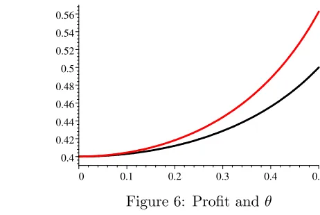
prominence difference between firms will benefit both firms. The intuition is, when more consumers consider product 1first,firm 1 will rely more on those strong-taste consumers and so charge the high price more frequently, which will further relax the price competition in an environment where prices are strategic complements. Figure 6 below is a numerical example withλ = 2. For a general distribution, we have the same result at least in the limit case withλ close to one.36

0.4 0.42 0.44 0.46 0.48 0.5 0.52 0.54 0.56

0 0.1 0.2 0.3 0.4 0.5

Figure 6: Profit andθ

3 4_{The advertising story also applies to the case in which the platform can sell prominent placements to}

firms.

3 5_{This is because the derivative of the bracket term with respect toθ has the sign of} 1

l√l−

1

h√h >0.

One can further show that both profit functions are convex inθ.

3 6_{When λ= 1 +ε and εtends to zero, using the approximations in footnote 24, we can approximate}

equilibrium profits asπ1≈p₂ + (3₂θ2−1₄)pε2 andπ2≈ p₂+ (θ2−1₄)pε2. Both of them are increasing and

Given such a result, the answer to the platform story is easy to see: the platform will make one product more prominent than the other. Now let us consider the advertising-competition story. If advertising advertising-competition occurs prior to price advertising-competition and the ad-vertising technology is symmetric amongfirms, then two observations immediately follow. First, bothfirms advertising at the same positive level is not an equilibrium outcome. This is because otherwise eachfirm could then improve profit by reducing advertising unilater-ally. Second, if the twofirms advertise at different intensities, then thefirm advertising less must actually not advertise at all. Otherwise, it could always increase profit by reducing advertising and further enlarging the prominence difference. Thus, if we focus on pure-strategy advertising equilibrium, the two firms will either differentiate their advertising intensities (i.e., one advertises and the other does not) or both not advertise. Furthermore, if advertising is not too costly, the latter can neither be an equilibrium outcome, which leaves asymmetric advertising as the only possible pure-strategy equilibrium. Hence, con-sumer reference dependence might give rise to endogenous asymmetric prominence as a result of advertising competition.37

5

Reference Dependence and Product Qualities

We now return to the setting with exogenous prominence and explore how consumer reference dependence could shape firms’ product quality choices. We will first study the properties of equilibrium with two products differing in their qualities. The mainfinding is, when mixed-strategy equilibrium occurs, a relative increase of the prominent product’s quality will soften price competition and benefit bothfirms. We then deduce that the less prominent firm may want to choose a lower quality level than its prominent rival even if improving quality is costless.

Letvi be product i’s gross utility, and define 4=v1−v2 to be the quality difference

between the two products. We assume that firm 1 is exogenously more prominent and

1

2+θof consumers will consider itfirst. Denote byxˆthe solution tov1−x=v2−(1−x).

Then the consumer at

ˆ

x= 1 2 +

4

2

is indifferent between the two products if there is no price difference. To make the situation interesting, we focus on mild quality difference 4 ∈ (−1,1) such that xˆ ∈ (0,1). That is, no firm will occupy the whole market if they charge the same price. For tractability, we focus on the uniform setting again. One can check that now the demand functions become38

q1= ˆx+

i

2(p2−p1), q2 = 1−xˆ+

i

2(p1−p2), wherei=h ifp1 < p2 and i=l ifp1 > p2.

3 7_{It is straightforward to write down a formal model of advertising competition in which we can show}

the existence of pure-strategy advertising equilibrium under certain conditions. We can also discuss the properties of possible mixed-strategy advertising equilibrium. The details are available from the author.

3 8_{We are implicitly assuming that consumers regard personal taste and product quality together as the}

We derive equilibriumfirst. Now the equilibrium will be either pure-strategy or mixed-strategy depending on the magnitude of quality difference relative to the strength of ref-erence dependence. If there is no consumer refref-erence dependence and4>0, clearlyfirm 1 will charge a higher price than firm 2. When the psychological bias emerges, charging a lower price than its rival will also become an attractive strategy tofirm 1, because that will expand its market share substantially (rememberfirm 1 is more prominent). Hence, we expect that, forfixed quality difference, when the psychological bias becomes stronger gradually, the equilibrium should evolve from a pure-strategy one to a mixed-strategy one. Let us keep the notationr=qh_l which increases with λandθ, and define

a(x) = 2−x

x ; b(x) = 3

r

1−x

5₋5x₋x2.

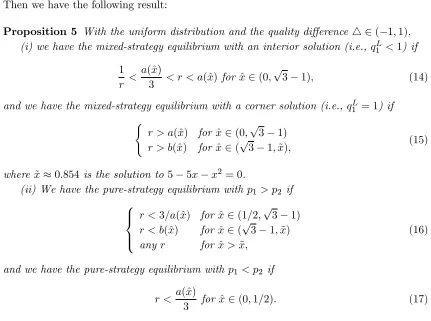
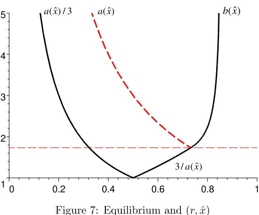
Then we have the following result:

Proposition 5 With the uniform distribution and the quality difference4_∈(₋1,1), (i) we have the mixed-strategy equilibrium with an interior solution (i.e., q₁L<1) if

1

r < a(ˆx)

3 < r < a(ˆx) for xˆ∈(0,

√

3₋1), (14)

and we have the mixed-strategy equilibrium with a corner solution (i.e.,qL

1 = 1) if

(

r > a(ˆx) for xˆ∈(0,√3−1)

r > b(ˆx) for xˆ_∈(√3₋1,x˜), (15)

where x˜_≈0.854is the solution to 5₋5x₋x2 _{= 0.}

(ii) We have the pure-strategy equilibrium with p1> p2 if

⎧ ⎪ ⎨ ⎪ ⎩

r <3/a(ˆx) for xˆ_∈(1/2,√3₋1)

r < b(ˆx) for xˆ∈(√3−1,x˜) anyr for x >ˆ x,˜

(16)

and we have the pure-strategy equilibrium withp1 < p2 if

r < a(ˆx)

3 / ) ˆ (x

a a(xˆ) b(xˆ)

3/a(xˆ)

₁

2 3 4 5

0 0.2 0.4 0.6 0.8 1

Figure 7: Equilibrium and(r,xˆ)

In the area below the solid lines, we have pure-strategy equilibrium. In the area above them, we have mixed-strategy equilibrium. This area is further divided by the dashed line

a(ˆx). Below that, we have the interior-solution equilibrium, and above that, we have the corner-solution equilibrium. Whenr <√3(i.e., below the horizontal dashed line), there is no mixed-strategy equilibrium with a corner solution for anyxˆ. We observe that, forfixed

r, mixed-strategy equilibrium is more likely to occur for smaller quality difference; and for

fixed x <ˆ x˜≈ 0.854, mixed-strategy equilibrium is more likely to occur for greater r (so for greater θor λ). (In particular, when there is no quality difference (i.e., when xˆ= 1₂), we only have mixed-strategy equilibrium.) These two observations illustrate Proposition 3.

We now turn to investigate the properties of equilibrium. In the pure-strategy equi-librium, we can show

p1 = 2

i ·

1 + ˆx

3 , π1 = 2

i

µ

1 + ˆx

3

¶2

;

p2 =

2

i ·

2−xˆ

3 , π2 = 2

i

µ

2−xˆ 3

¶2

,

wherei=l if x >ˆ 1₂ and i=h if x <ˆ 1₂. It is clear that p1 and π1 increase with xˆ while

p2 and π2 decrease withxˆ. Thus, a relative increase offirm 1’s quality will benefit firm 1

but hurtfirm 2. This is consistent with the result in the orthodox model withλ= 1. However, the situation is very different in the mixed-strategy equilibrium. Our discus-sion is based on the interior-solution case. (In Appendix A.5 we establish the similar results in the corner-solution case.) First, from (33) and (34), we see thatall prices increase with ˆ

x and μ decreases with xˆ (i.e., firm 1 will charge the high price more frequently when its relative quality rises). Second, following the proof of Proposition 5, simple calculation yields

π1=

(1 +r)2

2h xˆ

2_{, π} 2=

2r

3h(2−xˆ)ˆx.

The results concerning firm 1 are not surprising, and here we try to understand the results concerning firm 2. When firm 1’s relative quality increases, several forces affect

firm 2’s pricing incentive. Let us see itsfirst-order condition p2 =q2e/(− ∂qe

2

∂p2), where qe2 is

its expected demand defined in (32). (i) Given prices, higher xˆ reduces qe

2 directly since

firm 2 is then relatively less favored by consumers. This will drive firm 2 to lower its price. (ii) Higherxˆ causes higher prices offirm 1 and lowerμ, which will enhance qe

2 and

give firm 2 an incentive to raise its price. (Note that this is the standard strategic effect in an environment where prices are strategic complements.) (iii) Lowerμ also decreases

−∂q2e

∂p2 = 12(μh+ (1−μ)l) (i.e., makes firm 2’s expected demand less price responsive).

This is because consumers in aggregate are less price sensitive when firm 1 charges the high price. This will further motivate firm 2 to raise its price. The first two effects are standard, but the third one is only present in the mixed-strategy equilibrium caused by consumers reference dependence. Our result implies that the latter two positive effects together outweigh the first negative one. In light of this price result, the profit result is not difficult to understand.

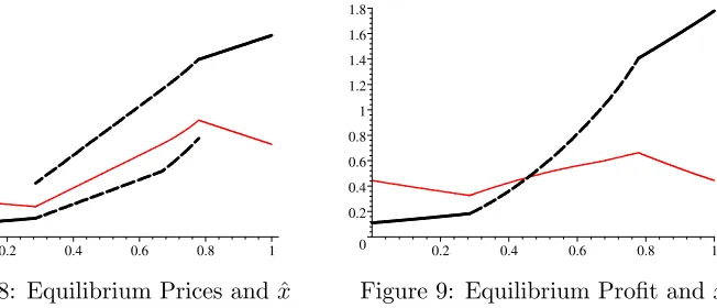
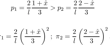
We further illustrate the above results in the following two graphs which are based on a numerical example withθ= 1₂ and λ= 2.

0.5 1 1.5 2 2.5

0 0.2 0.4 0.6 0.8 1

Figure 8: Equilibrium Prices and xˆ

0 0.2 0.4 0.6 0.8 1 1.2 1.4 1.6 1.8

0.2 0.4 0.6 0.8 1

Figure 9: Equilibrium Profit andxˆ

They describe how equilibrium prices and profit vary withxˆ, respectively. (The thick lines correspond tofirm 1, and the dashed parts correspond to the mixed-strategy equilibrium.) The main implication of the above results is, when the quality difference between the two products is not too large (such that the mixed-strategy pricing equilibrium occurs), the less prominentfirm hasnoincentive to improve its quality slightly even if it is costless to do so. This is because it does not want to trigger the prominentfirm to charge a low price more frequently. Put differently, the less prominent firm even has an incentive to reduce its quality even if doing so does not save any costs. We then deduce, if onefirm is more prominent than the other and if there is a (simultaneous) quality choice stage before the price competition, choosing the same positive quality level will never be an equilibrium outcome. This is because atxˆ= 1₂ we must have the mixed-strategy equilibrium and then

π2 increases with xˆ (i.e., reducing quality is profitable for firm 2). This also implies, at

level than its prominent rival even if improving quality is costless.39,40

We summarize the main results in the following proposition:

Proposition 6 (i) With the uniform distribution and product 1’s relative quality “advan-tage”4∈(−1,1), the prominent firm 1’s prices and profit always increase with4. Firm 2’s price and profit decrease with 4 in the pure-strategy equilibrium, but increase with 4

the mixed-strategy equilibrium.

(ii) Suppose there is a quality choice stage prior to the price competition. Then in equilibrium the twofirms will never choose the same quality level. Moreover, at least when the range of feasible quality levels is relatively narrow, the less prominentfirm will choose a lower quality level than its prominent rival even if improving quality is costless.

Discussion:

The reference-dependence effect in our model can be regarded as a kind of switching cost. But it occurs only if the second product is relatively inferior to the first one in at least one aspect. Readers may wonder whether the results we have derived in this paper could be replicated by using an exogenous cost involved in moving from one product to the other. In that setting, all else equal, the prominentfirm will also earn more than the other, but we cannot establish other main results. Suppose the cost is s. Then, with the same notation, the demand functions are:

q1(p1) = ˆx+θs+

p2−p1

2 ; q2(p2) = 1−(ˆx+θs) +

p1−p2

2 .

Since they are smooth functions, nofirm will randomize its price. If sis appropriate such that we have an interior-solution equilibrium, then the equilibrium prices and profits are:

p1 =

2

3(1 + ˆx+θs), π1 = 2

9(1 + ˆx+θs)

2_;

p2 = 2

3(2−xˆ−θs), π2 = 2

9(2−xˆ−θs)

2_.

Clearly, making onefirm more prominent or improving its product quality will benefit this

firm but harm the other, so our results on advertising and quality choice will not emerge either.

6

Conclusion

This paper has examined the impacts of consumer reference dependence on market com-petition. In particular, if consumers take somereal product in the market as the reference point and exhibit loss aversion, thefirm whose product is more likely to be taken as the

3 9_{This result could even hold for a broader range of quality levels. Let us see the following simple}

example. Suppose the free quality feasible set isvi∈[v, v+ 1](so4∈[−1,1]). Then it is clear that the

prominentfirm 1 will always pick the highest quality levelv1=v+ 1. Firm 2’s problem is thus to choose

ˆ

xbetween[1₂,1]. From Figure 9, we see that it will choose xr > 1₂ (i.e.,v2< v1), wherexr is the upper

limit value ofxˆsuch that we have a mixed-strategy pricing equilibrium atr.

4 0