U.S. Wage and Price Dynamics: A
Limited-Information Approach
Sbordone, Argia M
12 July 2006
A Limited-Information Approach
∗Argia M. Sbordone
Federal Reserve Bank of New York
This paper analyzes the dynamics of prices and wages using a limited-information approach to estimation. I estimate a two-equation model for the determination of prices and wages derived from an optimization-based dynamic model, where both goods and labor markets are monopolistically competi-tive, prices and wages can be reoptimized only at random inter-vals, and, when not reoptimized, can be partially adjusted to previous-period aggregate inflation. The estimation procedure is atwo-step minimum-distance estimation, which exploits the restrictions that the model imposes on a time-series represen-tation of the data. In the first step I estimate anunrestricted autoregressive representation of the variables of interest. In the second step, I express the model solution in the form of a con-strained autoregressive representation of the data and define the distance between unconstrained and constrained represen-tations as a function of the structural parameters that char-acterize the joint dynamics of inflation and labor share. This function summarizes the cross-equation restrictions between the model and the time-series representations of the data: I then estimate the parameters of interest by minimizing a quadratic function of that distance. I find that the estimated dynamics of prices and wages track actual dynamics quite well, and that the estimated parameters are consistent with the observed length of nominal contracts.
JEL Codes: E32, C32, C52.
∗I wish to thank the editor John B. Taylor and coeditor Frank Smets for
their detailed comments and suggestions. I also wish to thank Jean Boivin, Marc Giannoni, Ken Kuttner, Bruce Preston, Mike Woodford, and seminar participants at the 2005 Annual Meeting of the Society for Computational Economics, the
1. Introduction
This paper is an empirical analysis of the dynamics of wages and prices implied by a model of monopolistic competition in goods and labor markets, with sluggish adjustment of prices and wages. The objective of the paper is to investigate the link between real and nominal variables predicted by an optimization-based model, without specifying the whole general equilibrium structure.
I build on previous work that has shown that inflation fluctu-ations are fairly consistent with the predictions of an optimizing model of staggered price setting, if one takes as given the evolution of marginal cost.1I take the analysis one step further, endogenizing the determination of nominal wages, to provide an empirical analy-sis of the joint dynamics of wages and prices and their interaction with aggregate real variables. Allowing sluggish adjustment of both wages and prices, I also seek to shed light on whether the source of the inertia that appears to characterize nominal variables rests more on the price or on the wage-adjustment mechanism.
I analyze a generalized version of the discrete-time model of price and wage setting studied by Erceg, Henderson, and Levin (2000).2 Specifically, I assume that monopolistically competitive goods-producing firms set their prices to maximize the discounted expected value of their future profits and reoptimize prices only at
Structural Analysis Division of the Bank of England, the Ente Einaudi in Rome, Barnard College, the Graduate School of Business at Columbia University, and the Research Departments of the Federal Reserve Bank of New York and the Federal Reserve Bank of Chicago. The views expressed in this paper do not nec-essarily reflect the position of the Federal Reserve Bank of New York or the Federal Reserve System. Author contact: Research and Statistics Group, Federal Reserve Bank of New York, 33 Liberty Street, New York, NY 10045; Tel: (212) 720-6810; e-mail: [email protected].
1
This is argued by Gal´ı and Gertler (1999), Gal´ı, Gertler, and L´opez-Salido (2005), and Sbordone (2002) for the United States; and Gal´ı, Gertler, and L´ opez-Salido (2001), Batini, Jackson, and Nickell (2005), and Gagnon and Khan (2005) for European countries and Canada. The robustness of these estimates has been variously discussed: among the criticisms, see Rudd and Whelan (2005), Kurmann (2005), and Lind´e (2005).
2
random intervals. Similarly, monopolistically competitive suppliers of differentiated labor services can reoptimize their wages only at random intervals. On the other hand, I assume that both firms and workers, when not allowed to reoptimize, can adjust their prices to past inflation.
Sluggish price and wage adjustments of this kind, following Calvo (1983) modeling, are often introduced in general equilibrium models of business cycle to build in a channel of persistence of monetary policy effects. Estimating the price/wage block within a completely specified general equilibrium model requires further specifications, such as the nature of capital accumulation, the details of fiscal and monetary policy, and the stochastic properties of the shocks. Some papers do so by adopting a full-information approach to estima-tion using maximum likelihood methods;3 others rely on the iden-tification of a single shock and estimate the model parameters by matching theoretical and empirical impulse response functions to that shock.4
The strategy I propose here aims instead at estimating the dynamics of wages and prices implied by this model without specify-ing a whole general equilibrium structure. I compare the equilibrium paths of wages and prices derived from the optimizing model to the paths described by an unrestricted vector autoregression model. Under the null hypothesis that the theoretical model is a correct representation of the stochastic process generating the data, the restrictions that the model solution imposes on the parameters of the time-series model should hold exactly. I propose to use these restric-tions to construct a two-step distance estimator for the parameters of the structural model.
This approach follows directly from Campbell and Shiller’s (1987) analysis, where they suggested testing the present-value model of stock prices by testing the restrictions that it imposes on a bivariate time-series representation of dividends growth and the price/dividend ratio. The model analyzed here also involves two
3
For small models, the pioneering work using maximum likelihood estimation is Ireland (1997). Smets and Wouters (2003, 2005) have introduced the use of Bayesian techniques in the estimation of medium-scale models.
4
present-value relationships. In the price equation, after solving out inflation expectations, price inflation depends upon the present dis-counted value of expected future deviations of marginal costs from the price level. Similarly, after solving forward wage expectations in the wage equation, wage growth depends upon the present dis-counted value of expected future deviations of the marginal rate of substitution from the real wage. The joint model therefore imposes testable restrictions on a multivariate time-series representation of wages and prices.
My estimation approach proceeds as follows. I derive the (approx-imate) equilibrium conditions for price and wage setting from the optimization-based model and write them in the form of two expec-tational difference equations in inflation and labor share. I then esti-mate a multivariate time-series model to describe the evolution of all the variables that matter in the determination of inflation and labor share. Combining the structural equations and the estimated time-series model, I solve for the paths of inflation and labor share as functions of exogenous and predetermined variables. This solution represents arestricted autoregressive representation for inflation and labor share, where the parameters are combinations of the struc-tural parametersand the parameters of the unrestricted time-series process. I then recover the restrictions imposed by the theoretical model by comparing the coefficients of the restricted and the unre-stricted autoregressive representations. These implied restrictions can be interpreted as a measure of the distance between the model and the time-series representation: the structural parameters are estimated as those that minimize a quadratic form of this distance. The estimator I propose is therefore a two-step distance estima-tor: the first step involves the estimation of the time-series model, and the second, taking as given those estimated parameters, mini-mizes the distance function.
The second issue is modeling the marginal rate of substitution, which is the real wage that would prevail in a competitive market, absent wage rigidities; throughout the paper I refer to the marginal rate of substitution as the flexible-wage equilibrium real wage. The expression for this equilibrium wage depends upon the assumptions that one makes about household preferences; without adopting spe-cific functional forms for preferences, I discuss in turn the form that the flexible-wage equilibrium real wage would take under different assumptions.
The rest of the paper is organized as follows. In section 2, I lay out the elements of the optimization model for the determination of the path of price and wage inflation. In section 3, I characterize the model solution; in section 4, I describe the two-step estimator, relating it to similar estimation approaches used in business-cycle literature. Section 5 discusses how to model the flexible-wage equi-librium real wage, while section 6 presents the estimation of the time-series model and discusses the treatment of the trend. Results are presented and discussed in section 7. After a brief discussion of robustness checks in section 8, section 9 concludes.
2. Wage and Price Dynamics with Backward Indexation
The model is based on Erceg, Henderson, and Levin (2000), but allows partial indexation of both wages and prices to lagged infla-tion.5 Since the basic structure of this model is quite well known in the literature, the exposition below is kept to a minimum6 and targeted to illustrate the coefficients to be estimated.
2.1 Staggered Price Setting with Partial Indexation
At any point in time, a fraction (1−αp) of the firms choose a price
Xptthat maximizes the expected discounted sum of the firms’ profits
EtΣjαjpQt,t+j(XptΨtjYt+j(i)−C(Yt+j(i)), (1)
5
Full backward indexation was first introduced in Christiano, Eichenbaum, and Evans (2005). The generalized model with partial backward indexation is detailed in Woodford (2003, ch. 3).
6
where Qt,t+j is a nominal discount factor between timetandt+j;
Yt(i) is the level of output of firm i;C(Yt+j(i)) is the total cost of
production at t+j of the firms that optimally set prices at t; and
Ψtj =
1 j= 0
Πj−1
k=0π
̺p
t+k j≥1
. (2)
The coefficient ̺pǫ[0,1] indicates the degree of indexation to past inflation of the prices that are not reoptimized.
The demand for goods of produceriis
Yt+j(i) =
XptΨtj
Pt+j
−θp
Yt+j, (3)
where θp > 1 denotes the Dixit-Stiglitz elasticity of substitution among differentiated goods, and the aggregate price level is
Pt=
,
(1−αp)X
1−θp
pt +αp(πt̺−p1Pt−1)1−θp
- 1 1−θp
. (4)
The first-order condition for this problem can be expressed as
EtΣjαjpQt,t+j
.
Yt+jPtθ+pjΨtj1−θp
Xpt− θp
θp−1
St+j,t(i)Ψ −1
tj
/
= 0,
whereSt+j,t(i) is nominal marginal cost att+jof the firms that set
optimal price at time t. Dividing this expression by Pt, and using
(2), one gets
EtΣjαjpQt,t+j
.
Yt+jPtθ+pjΨtj
1−θp
×
xpt−
θp
θp−1st+j(i)
Πjk=1πt+k Πj −1
k=0π
̺p
t+k
−1/ = 0,
where xpt is the relative price of the firms that set optimal price at t, and st+j,t(i) is their real marginal cost at time t+j. A
log-linearization of this expression around a steady state with zero inflation gives
ˆ
xpt= (1−αpβ)Σj∞=0(αpβ)jEt
ˆ
st+j,t+ Σjk=1πˆt+k−̺pΣj −1 k=0ˆπt+k
,
where hat variables are log-deviations from steady-state values.7 Under the hypothesis that capital is not instantaneously reallocated across firms,st+j,t is, in general, different from the average marginal
cost at timet+j, st+j, so that
ˆ
st+j,t= ˆst+j −θpω
ˆ
xpt−
Σjk=1πˆt+k−̺pΣj −1
k=0πˆt+k
, (6)
where ω is the output elasticity of real marginal cost for the indi-vidual firm.8 Therefore, substituting (6) in (5), one obtains
(1 +θpω)ˆxpt= (1−αpβ)Σ∞j=0(αpβ)j
×Et
ˆ
st+j + (1 +θpω)
Σjk=1ˆπt+k−̺pΣj −1
k=0πˆt+k
.
(7)
Similarly, dividing (4) byPt and log-linearizing, one gets
ˆ
xpt= αp 1−αp
(ˆπt−̺pπˆt−1). (8)
Finally, combining (7) and (8),
ˆ
πt−̺pπˆt−1=
(1−αp)(1−αpβ)
αp(1 +θpω)
Σ∞
j=0(αpβ)j
×Et
ˆ
st+j + (1 +θpω)
Σjk=1ˆπt+k−̺pΣj −1
k=0πˆt+k
,
(9)
which is equivalently written as9
ˆ
πt−̺pπˆt−1=ζˆst+βEt(ˆπt+1−̺pπˆt),
7
I denote byβthe steady-state value of the discount factor and suppress the indexion variables chosen by the firms that are changing prices, since all those firms solve the same optimization problem.
8
Note that when the production function takes the Cobb-Douglas form, for example, ω=a/(1−a),where (1−a) is the output elasticity with respect to
labor.
9
where I setζ = (1−αp)(1−αpβ)
αp(1+θpω) .This equation describes the evolution
of inflation as a function of past inflation, expected future inflation, and real marginal costs; compared to the standard Calvo model, where ̺p = 0, this expression contains a backward-looking
compo-nent that many have argued is a necessary compocompo-nent to fit the inertia of inflation data. This can be seen by rewriting (9) as:
ˆ
πt=
̺p
1 +̺pβ
ˆ
πt−1+
β
1 +̺pβ
Etπˆt+1+
ζ
1 +̺pβ
ˆ
st. (10)
At the other extreme of complete indexation (̺p = 1)—considered,
for example, in Christiano, Eichenbaum, and Evans (2005)—the model predicts that the growth rate of inflation depends upon real marginal costs and the expected future growth rate of inflation. In this case, coefficients on past and future inflation sum to 1, and, forβ close to 1, they are approximately the same. For low levels of indexation, instead, the coefficient on past inflation is significantly smaller than the one on future inflation.10
2.2 Staggered Wage Setting with Partial Indexation
Similarly to the firms, households are assumed to set their price (for leisure) in a monopolistically competitive way, analogous to the price model. Each household (indexed byi) offers a differentiated type of labor services to the firms and stipulates wage contracts in nominal terms: at the stipulated wage Wt(i) they supply as many hours as
are demanded. Unlike Erceg, Henderson, and Levin (2000), however, I allow preferences to be nonseparable in consumption and leisure.11 Total labor employed by any firmjis an aggregation of individual differentiated hours ht(i)
Htj =
1
0
ht(i)(θw−1)/θwdi
θw/(θw−1)
, (11)
10
An equation of similar form is obtained with a slightly different set of assump-tions by Gal´ı and Gertler (1999). They assume that part of the firms that reset their price are not forward looking, but adopt instead “rule-of-thumb” price setting.
11
whereθw is the Dixit-Stiglitz elasticity of substitution among
differ-entiated labor services (θw >1). The wage index is an aggregate of individual wages, defined as
Wt =
1
0
Wt(i)1−θwdi
1/(1−θw)
.
The demand function for labor services of household i from firm
j is12
hjt(i) = (Wt(i)/Wt)−θwHtj, (12)
which, aggregated across firms, gives the total demand of labor hours
ht(i) equal to
ht(i) = (Wt(i)/Wt)−θwHt, (13)
whereHt= 01Htjdj.
At each point in time, only a fraction (1 −αw) of the
house-holds can set a new wage, which I denote by Xwt, independently
of the past history of wage changes.13 The expected time between wage changes is therefore 1−1α
w. I also assume, as in Erceg,
Hender-son, and Levin (2000), that households have access to a complete set of state-contingent contracts; in this way, although workers that work different amounts of time have different consumption paths, in equilibrium they have the same marginal utility of consumption.
Finally, for wages that are not reoptimized, I allow indexation to previous-period inflation: specifically, for̺wǫ[0,1], the wage of a householdl that cannot reoptimize att evolves as
Wt(l) =πt̺−w1Wt−1(l).
This hypothesis implies that wages reset at time t are expected to grow during the contract period according to
Xwt+j =XwtΨwtj, where Ψwtj =
1 ifj= 0
0j−1 k=0π
̺w
t+k ifj≥1
. (14)
12
This demand is obtained by solving firmj’s problem of allocating a given wage payment among the differentiated labor services, i.e., the problem of max-imizing (11) for a given level of total wages to be paid.
13
The aggregate wage at any time t is an average of the wage set by the optimizing workers, Xwt, and the one set by those who do not optimize:
Wt=
(1−αw)(Xwt)1−θw+αw(π̺t−w1Wt−1)1−θw
1
1−θw . (15)
The wage-setting problem is defined as the choice of the wage Xwt
that maximizes the expected stream of discounted utility from the new wage; this is defined as the difference between the gain (mea-sured in terms of the marginal utility of consumption) derived from the hours worked at the new wage and the disutility of working the number of hours associated with the new wage. The objective function is then
Et
Σ∞
j=0(βαw)j
Λc t+j,t
Pt+j
XwtΨwtjht+j,t−Pt+jCt+j,t
+U(Ct+j,t, ht+j,t)
, (16)
where Λc
t+j,t is the marginal utility of consumption att+j of
work-ers that optimize att, andht+j,tis hours worked att+j at the wage
set at timet. Given (14), the latter evolves as
ht+j,t=
X
wtΨwtj
Wt+j
−θw
Ht+j. (17)
The first-order condition for this problem can be written as
Et
Σ∞
j=0(βαw)j
X
wtΨwtj
Wt+j
−θw
Ht+j
X
wtΨwtj
Pt+j
− θw
θw−1
vt+j,t
= 0,
(18)
where vt+j,t is the marginal rate of substitution between
consump-tion and leisure at date t+j, when the level of hours is ht+j,t.
A log-linear approximation of this equation is14
ˆ
πtw−̺wˆπt−1=γ(ˆvt−ωˆt) +β
Etˆπwt+1−̺wπˆt
, (19)
14
where γ = (1−αw)(1−βαw)
αw(1+θwχ) ,and the parameter χ reflects the degree
of nonseparability in preferences.15
2.3 A Complete Model
The dynamics of wages and prices are then described by the two log-linearized equilibrium conditions (10) and (19). Because the approx-imations are taken around a point with zero wage and price inflation, ˆ
πt=πt≡∆pt,and ˆπtw=πwt ≡∆wt.Furthermore, ˆst=wt−pt−qt,
since real wage (wt−pt) and labor productivity (qt) share the same stochastic trend.16 Similarly, ˆv
t−ωˆt=vt−(wt−pt),since marginal
rate of substitution and real wage also share the same stochastic trend.
Equations (10) and (19) can then be rewritten as
πt=
̺p
1 +̺pβ
∆pt−1+
β
1 +̺pβ
Et∆pt+1
+ ζ
1 +̺pβ
((wt−qt)−pt) +upt (20)
πtw=̺w∆pt−1+βEt(∆wt+1−̺w∆pt)
+γ(vt−(wt−pt)) +uwt. (21)
These equations show that the dynamics of prices and wages are dri-ven by twogaps: the excess of unit labor costs over price (the real marginal cost) and the excess of the “equilibrium” real wage over the actual wage. The two parameters ζ and γ, defined quite sym-metrically as ζ = (1−αp)(1−αpβ)
αp(1+θpω) and γ =
(1−αw)(1−βαw)
αw(1+θwχ) , measure
the degree of gradual adjustment of prices and wages to these gaps. These parameters, in turn, depend upon the parameters that deter-mine the frequency of price and wage adjustments—respectively,αp
15
χ=−Λc hH
Λc
cC ηc+ηh, where ηc and ηh are, respectively, the elasticity of the
marginal rate of substitution with respect to consumption and with respect to hours, evaluated at the steady state. Λc
c and Λch are derivatives of the marginal utility of consumption Λcwith respect to consumption and with respect to hours, also evaluated at steady state. Note that when preferences are separable in con-sumption and leisure, Λc
h= 0.
16
andαw; the degree of substitutability between differentiated goods
θp and that between differentiated labor services θw; the elasticity of firms’ marginal costs with respect to their own outputω; and the degree of nonseparability in households’ preferences,χ.
I have included an error term in each equation: these terms may pick up unobservable markup variations or allow for other possible misspecifications. I assume that the error terms are mutually uncor-related, serially uncorrelated: E(uitu′jt−k) = 0 for i, j = p, w, and
k= 0,and unforecastable, given the information set.
Equations (20) and (21) show the interdependence of wages and prices and their dependence upon the evolution of productivity and the other real variables that determine the evolution of the flexible-wage equilibrium real flexible-wage. In a fully specified model, this evolution would be described by similar structural relations. Here, instead, I focus on the restrictions that these equilibrium conditions impose on any general model that includes sluggish price and wage adjust-ment of the form described, independently of the specific form that the other structural relationships may take.
I proceed as follows: I assume that the evolution of the variables that determine the path of wages and prices can be summarized by a covariance stationary m-dimensional processXt:
Xt = Φ1Xt−1+· · ·+ ΦpXt−p+εt (22)
(for some lag p to be determined empirically), where E(εt) = 0,
and E(εtε′τ) = Ω for τ = t and 0 otherwise. This vector includes,
in addition to wages and prices, labor productivity q and the determinants of the flexible-wage equilibrium real wage v. Letting
Zt = [XtXt−1. . . Xt−p+1]′, (22) can be represented as a first-order autoregressive process:
Zt =AZt−1+Qεt, (23)
where
A(mp×mp) =
⎡
⎣
Φ1 Φ2 · · · Φp−1 Φp
I 0 · · · 0 0
0 0 I 0
⎤
⎦, Q=
Im×m
0m(p−1)×m
.
can be recovered as follows: if one considers the joint process of (20), (21), and (23), one can solve for equilibrium processes{wt, pt}, given stochastic processes for {vt, qt} and initial conditions {w−1, p−1}. This solution can be expressed as a particular restricted reduced-form representation for the vectorZt,
Zt=ARZt−1+εt,
withAR=G(ψ, A). ψ is the vector of the structural parameters of
interest (defined below), and the functionGincorporates the restric-tions that the theoretical model imposes on the parameters of the time-series representation. The estimation procedure that I present in the next section is based on minimizing the distance between the restricted and the unrestricted representations of the relevant components of vector Zt (i.e., the relevant elements of matrices A
andAR).
Before discussing my implementation of this estimation pro-cedure, I will present a further transformation of equations (20) and (21) from equations in price and wage inflation into equations for price inflation and labor share (that is, real wage adjusted for productivity).17 I will also derive the specific form of the restric-tions that define the distance function used for the estimation of the structural parameters.
In what follows, I’ll make use of the following identities:
qt=qt−1+ ∆qt (24)
wt−pt=wt−1−pt−1+ ∆wt−∆pt (25)
and of an expression that defines the theoretical model for the flexible-wage equilibrium real wage:
vt=qt+ ΞZt. (26)
The elements of the matrix Ξ depend upon assumptions about the long-run trend driving the time series and the specification of the
17
unrestricted representation (23). The crucial assumption that deliv-ers (26) is that productivity, real wage, output, and consumption are all driven by a single stochastic trend, while hours are trend stationary. The specification of the vector Xt, the choice of the lag
length p, and the form of the vector of coefficients Ξ are discussed later.
3. Model Solution
To rewrite equations (20) and (21) as a system in inflation and labor sharest≡wt−pt−qt, I first rearrange equation (20) as
Et∆pt+1=
1 +̺pβ
β ∆pt− ̺p
β ∆pt−1− ζ
β(wt−pt−qt) +upt, (27)
where upt = (1 +̺pβ)β−1upt. Then I substitute (26) in (21) and
rearrange it to get
Et∆wt+1= 1
β∆wt+̺w∆pt− ̺w
β ∆pt−1
+γ
β(wt−pt−qt)− γ
βΞZt+uwt, (28)
where uwt = β−1u
wt. Subtracting (27) and Et∆qt+1 from (28), I derive Et∆st+1≡Et(∆wt+1−∆pt+1−∆qt+1) as
Et(st+1−st) =
1
β∆wt+
̺w−̺p−
1
β
∆pt+
̺p−̺w
β
∆pt−1
+
γ+ζ β
st−
γ
βΞZt−Et∆qt+1+νt, (29)
where νt is a composite error term.18
As I explain below, productivity growth ∆qtis an element of the
vectorXt so that, by (23),
Et∆qt+1=e′qAZt, (30)
18
where the selection vector e′
q has a 1 in correspondence to
produc-tivity growth and 0 elsewhere. Combining the terms inst and using (30), equation (29) becomes
Etst+1= (̺w−̺p)∆pt+
1 +β+γ+ζ β
st+
̺p−̺w
β
∆pt−1
− 1
βst−1−
γ βΞ−
1
βe
′ q+e
′ qA
Zt+νt. (31)
I now define a vectoryt as
yt= [πt st πt−1st−1]′ (32)
and let Yt+1 = [yt+1 Zt+1]′. The system of equations composed of (27), (31), and (23) can then be written as
EtYt+1=M Yt+N ut, (33)
where ut = [upt uwt]′,and the matrices M (of dim. (4 +mp)) and
N are partitioned as follows:
M =
Myy MyZ
0 A
, N =
N1 0
.
The (4×4) blockMyydescribes the interaction of the structural
vari-ables; the (4×mp) blockMyZdescribes the dependence of structural
variables upon the exogenous block.19 If the matrixM has exactly two unstable eigenvalues, the system of equations (33) has a unique solution, which can be expressed in autoregressive form as
Yt=GYt−1+F υt, (34)
where the matrices G and F depend upon the vector of structural parametersψ and the parameters of the unrestricted VAR process, the elements of A; the error term is υt = (u′t, ε
′ t)
′
. The solution for
19
The matrixN1 is
β−1
(1 +̺pβ) 0
−β−1(1 +̺pβ) β−1
the endogenous variablesπt andst is the upper block of (34), which
can be expressed as
πt ≡y1t=gπ(ψ, A)Yt−1+fπυt=gπyyt−1+gZπZt−1+fπυt (35)
st ≡y2t=gs(ψ, A)Yt−1+fsυt =gsyyt−1+gZsZt−1+fsυt, (36)
where gi andfi (fori=π, s) denote the row of the matrices Gand
F corresponding to variable i.
4. Approach to Estimation
Since both inflation and labor share are elements of the unrestricted process (22), they can be expressed as elements of Zt, with
appro-priate definitions of selection vectors e′
π ande′s:
πt=e′πZt and st=e′sZt. (37)
Similarly, the components of vector yt−1, which includes lagged inflation and labor share, can be expressed in terms of elements of the vector Zt−1, by way of an appropriate selection matrix Υ : yt−1 = ΥZt−1. Using this definition, and substituting (37) in (35) and (36), I get
e′
πZt−gπyΥZt−1−gπZZt−1=fπυt (38)
e′
sZt−gysΥZt−1−gsZZt−1=fsυt. (39)
Finally, projecting both sides of (38) and (39) onto the information set Zt−1 and observing that, by assumption, E(υt|Zt−1) = 0, and also E(Zt|Zt−1) =AZt−1,I obtain
e′
πAZt−1−gyπΥZt−1−gZπZt−1= 0
e′
sAZt−1−gsyΥZt−1−gZsZt−1= 0.
Since these equalities must hold for every t, it follows that
e′
πA−gπyΥ−gZπ = 0 (40)
e′
sA−gsyΥ−gZs = 0. (41)
model is true. The structural parameters can then be estimated as those values that most likely make these restrictions hold.
The estimation strategy proceeds in two steps. First, I estimate an unrestricted VAR in all the variables of interest, to obtain a con-sistent estimate ˆAof the autoregressive matrixA. In the second step, taking as given the estimated matrix ˆA, and stacking the restrictions (40) and (41) in a vector function ̥(ψ, A) = 0,I choose the
struc-tural parametersψto make the empirical value of the function̥as
close as possible to its theoretical value of zero; namely, I choose
ˆ
ψ= arg min̥(ψ,Aˆ)′W−1̥(ψ,Aˆ) (42)
for an appropriate choice of the weighting matrixW.20
The proposed estimator can be interpreted as a minimum-distance estimator, in application of the approach that Campbell and Shiller (1987) proposed for the empirical evaluation of present-value models. I have in fact interpreted the restrictions that define the function̥ as measuring the “distance” between the restricted and
unrestricted representations of the data.21 This estimator is close in spirit to another distance estimator used in the business-cycle litera-ture, based on matching empirical and theoretical impulse response functions to specific structural shocks.22 That estimator, as the one proposed here, uses an auxiliary VAR model in the first stage to characterize the dynamics of the data; then it minimizes the dis-tance between the dynamic response to identified exogenous shocks estimated in the data and the response predicted by the theoretical model. Unlike the estimator based on matching impulse response
20
As weighting matrix, I use a diagonal matrix with the variance of the esti-mated parametersAalong the diagonal. This choice downweights the parameters that are estimated with greater uncertainty.
21
In my previous applications of a similar two-step minimum-distance estima-tion, the objective function had the form of an (unweighted) distance between “model” and data (Sbordone 2002).
22
functions, the one proposed here doesn’t rely on further identifica-tion restricidentifica-tions—those necessary to recover the structural shocks from the VAR innovations. Instead, it exploits the specific restric-tions that the VAR specification imposes on the solution of the structural model and tries to match the dynamic evolution of the endogenous variables implied by the theoretical model with their evolution as described by the data.
Finally, although the distance restrictions are not moments con-ditions, this estimator is similar to a GMM estimator whose instru-ments are the variables of the time-series representation. However, such an estimator is usually applied to orthogonality conditions that proxy the future values of the endogenous variables, as opposed to solving the expectational equations.23
5. Modeling the Flexible-Wage Equilibrium Real Wage
A crucial step in implementing the empirical strategy discussed is the specification of the flexible-wage equilibrium real wage. Relationship (26) expresses the theoretical link between the flexible-wage equilib-rium real wage (which I denoted by vt) and real variables in Zt
that are not determined by the two structural equations. Therefore, the expression for the parameter vector Ξ incorporates hypotheses about the determinants of the cyclical components of the marginal rate of substitution, together with hypotheses about the evolution of its trend component.
The real wage vt is the equilibrium wage that solves the
house-hold optimization problem under flexible wages: it is therefore equal to the ratio of the marginal disutility of working Λh
t and the
mar-ginal utility of consumption Λct. If there is no time dependence in the momentary utility function, these marginal utilities depend only upon current values of consumption and hours,24and a log-linearized expression for vt is
ˆ
vt=ηcˆct+ηhˆht, (43)
23
See my discussion of this point in Sbordone (2005).
24
where the coefficients ηi are elasticities. Since “hat” variables are
deviations from steady state, which are defined after appropriate transformations of the variables to remove their (possibly stochas-tic) trends, their natural empirical counterparts are cyclical compo-nents defined as deviations from estimated trends. Their derivation is explained in the next section.
6. The Time-Series Model
The second crucial step of the empirical methodology that I described is the specification of the unrestricted joint dynamics of the variables that appear as endogenous and forcing variables in the structural equations (20) and (21). These variables are inflation, labor share, labor productivity, and, following the discussion of the previous section, consumption and hours of work, which determine the evolution of the flexible-wage equilibrium real wage.
The first order of problems is choosing a transformation of the data consistent with the hypotheses built into the model. The time series of productivity, real wage, consumption, and output all contain a unit root, but it appears that the consumption-output ratio and the ratio of real wage to labor productivity are stationary. Hours, in turn, appear stationary around a deterministic trend. One can then assume that there is only one common stochastic trend to drive the long-run behavior of the series considered.
The hypothesis of a single stochastic trend in the data is con-sistent with the assumption built into the model that the economy is driven by a single source of nonstationarity.25 As in the model, stationary variables used in estimation are then defined as deviation from this single stochastic trend. I handle the nonstationarity in the same multivariate context that I use for the time-series represen-tation and apply the Beveridge-Nelson (1981) detrending method. The vectorXt of (22) is specified as
Xt= [∆qt ht cyt πt st]′, (44)
25
where ∆qt is labor productivity growth,ht is an index of hours,cyt
is the consumption output ratio, st is the share of labor in total output, and inflation is the rate of growth of the implicit GDP deflator.26
I use the fact that any difference stationary series can be decom-posed in a random-walk component (the stochastic trend) and a stationary component. I identify the single common stochastic trend in vectorXtwith the random-walk component of labor productivity,
which is in turn defined as the current value of productivity plus all expected future productivity growth.27 Formally, letting q
t denote
labor productivity, its trend is defined as
qTt = lim
k→∞
Et(qt+k−kµq) =qt+ ∞
j=1
Et(∆qt+j−µq), (45)
where µq = E(∆q). The stationary, or cyclical, component of
pro-ductivity is then defined as the deviation of the series from its sto-chastic trend. The assumption of stationary labor share in the VAR in turn implies that the trend in real wage is the same as the trend in productivity, and the stationarity of the consumption-output ratio, together with the stationarity of hours (which corresponds to the ratio of output to productivity), implies that consumption shares the same trend as productivity.
The cyclical variables that appear in the theoretical model can be constructed as deviations from their respective trends.28 From the joint representation of the series in (23), the s-step-ahead fore-casts that define the trend are easily computed, for each variable i
in vector X,as
EtXi,t+s =e′iEtZt+s =e′iAsZt. (46)
26
Unless otherwise indicated, lowercase letters denote natural logs.
27
The rationale is that, if productivity growth is expected to be higher than average in the future, then labor productivity today is below trend; vice versa, if productivity growth is expected to be below average, then productivity today is above trend.
28
These forecasts underlie the derivation of the vector of parameters Ξ in the expression for the real wage vt in (26).29 The specifica-tion of Ξ completes the specificaspecifica-tion of the system (33) used for the estimation of the structural parametersψ.
Using (46), the trend in productivity defined in (45) is
qtT =qt+e′q[I−A] −1
AZt. (47)
The cyclical component of consumption is derived using the fact that the output-productivity ratio and the consumption-output ratio are stationary so that output, productivity, and consumption share the same stochastic trend. Writingct= (ct−yt) + (yt−qt) +qt,I obtain
that
ccyct =ct−cTt =e′
cyZt+e′hZt−e′q[I−A] −1
AZt, (48) where I have also used the fact that hours are stationary, so that cyclical hours hcyct are simply the appropriate component of vec-torZt.
7. Results
7.1 VAR Specification
In the estimation I use quarterly data from 1952:Q1 to 2002:Q1, with data for 1951:Q2–1951:Q4 as initial values. Productivity, out-put, wages, prices, and hours are for the nonfarm business sector of the economy.30 Nominal wage is hourly compensation, and real wage is nominal wage divided by the implicit GDP deflator. Con-sumption is the aggregate of nondurables and services.31I fit a VAR with three lags32 to the vector X
t defined in (44) and estimate the
common trend as the trend in productivity defined in (47). As dis-cussed above, productivity, real wage, and consumption share the
29
The derivation of Ξ as a function of the exogenous variables in vectorZ is detailed in the “Empirical Implementation” section of the appendix.
30
The time series are downloaded from the Federal Reserve Economic Data (FRED) database at the Federal Reserve Bank of St. Louis.
31
All variables are in deviation from the mean, and hours are linearly detrended. I also remove, prior to estimation, a moderate deterministic trend that appears in the consumption-output ratio and the labor share.
32
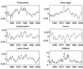
Figure 1. Real Variables: Cyclical Components (Inflation: Deviation from Mean, Annualized)
same stochastic trend, while hours have a deterministic trend. Sub-tracting the appropriate trends from the actual real series, I derive the series’ cyclical components, which I plot in figure 1. For inflation, the figure plots its deviation from a constant mean, annualized.
My objective is to compare the cyclical pattern of inflation and real wage to the pattern predicted by the theoretical model. As writ-ten, the model has implications for the dynamic behavior of inflation and labor share: given the behavior of productivity, the predicted path of real wages is then recovered from the estimated path of the labor share.
7.2 Estimation of Structural Parameters
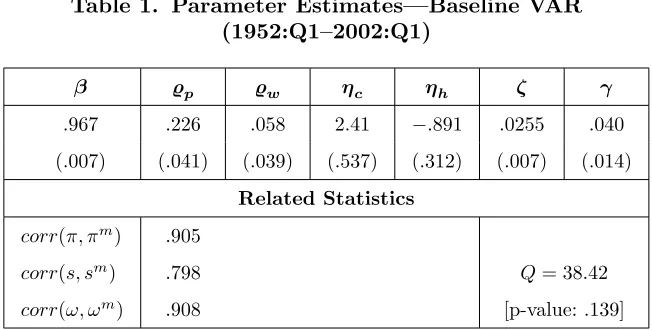
Recall that the parameter vector is
Table 1. Parameter Estimates—Baseline VAR (1952:Q1–2002:Q1)
β ̺p ̺w ηc ηh ζ γ
.967 .226 .058 2.41 −.891 .0255 .040
(.007) (.041) (.039) (.537) (.312) (.007) (.014) Related Statistics
corr(π, πm) .905
corr(s, sm) .798 Q= 38.42
corr(ω, ωm) .908 [p-value: .139]
where β is a discount factor; ̺p and̺w are indexation parameters,
respectively, for price and wage setting;ηc andηh are elasticities of
the marginal rate of substitution with respect to consumption and hours of work; andζ andγ are measures of the inertia in the price and wage settings. The last two parameters are nonlinear combina-tions of other structural parameters that are not separately identi-fied: the frequency of price and wage adjustments and the structure of technology and preferences. However, calibrating some of these parameters, we can draw some inference on which values of the frequency of price and wage adjustments are consistent with the estimated values ofζ andγ.
Table 1 reports parameter estimates, standard errors (in paren-theses),33 and correlation of the theoretical paths of inflation, labor share, and real wage (denoted with superscript m) with their observed counterparts.
33
To compute standard errors, I use the empirical distribution of the parameter matrixAto generateN samplesAi (i= 1, . . . , N): for each of these, I estimate a vector of structural parameters ˆψi.I then compute the sample variance of ˆψ and report the square root of its main diagonal elements as standard errors. For each estimated vector ˆψi, I also compute the value of the distance func-tion̥i and its covariance matrix Σ̥; the Wald statistic reported in the table
isQ=̥( ˆψ)′Σ
̥̥( ˆψ), where̥( ˆψ) is the value of the distance evaluated at the
Most of the estimated parameters are statistically significant. The parameters of the inflation model are consistent with sev-eral of the empirical results in the New Keynesian Phillips curve (NKPC) literature. First, there is a modest role for a backward-looking component in inflation dynamics: the indexation parameter
̺pis significantly different from zero, but the implied weight on the
backward-looking component (̺p/(1 +β̺p)≃.18) is quantitatively
much smaller than the weight on the forward-looking component (β/(1 +β̺p)≃.79).Secondly, the size of the coefficient on the labor share, as it will be discussed below, is consistent with other estimates of price inertia in the literature.
In the labor share equation, the parameter of wage indexation
̺wis much smaller than 1, the value imposed in Christiano,
Eichen-baum, and Evans (2005), and more in the range estimated by Smets and Wouters (2003) for the euro area. Finally, the value of the sta-tistic Q indicates that the restrictions that the model imposes on the parameters ofA cannot be rejected.
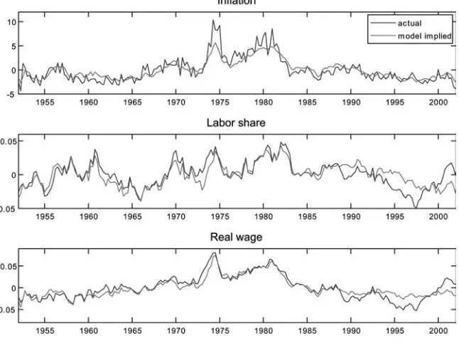
Figure 2 compares actual inflation, labor share, and real wage (namely, the cyclical components of these series as portrayed in figure 1) to the paths of inflation, labor share, and real wage con-structed recursively from the model solution evaluated at the esti-mated parameters—labeled “model implied” in the figure.34 These paths seem to capture well the underlying dynamics of the actual series: on these accounts, the model of wage and price inflation described seems to fit the data quite well.
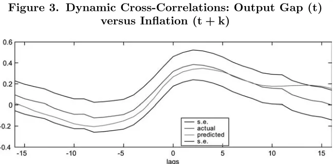
Furthermore, the model is able to match the dynamic corre-lation between inflation and output. As noted in the literature,35 output leads inflation in the data: the cyclical component of out-put, variously measured, is positively correlated with future infla-tion, with the highest value at about three quarters ahead. Purely forward-looking NKPCs driven by the output gap, when this is mea-sured as deviation from a deterministic trend, are unable to repro-duce such a result: output gap typically lags inflation in such a
34
The “model implied” paths of inflation and labor share are directly computed from expressions (35) and (36); the path of real wage is recovered from that of the labor share by adding productivity.
35
Figure 2. Inflation, Labor Share, and Real Wage: Actual versus Model Implied
model.36 Output-inflation correlations are shown in figure 3. The figure compares the dynamic correlation of output gap and actual inflation (the line labeled “actual”) with the dynamic correlation of output gap and the inflation series generated by the estimated model (the line labeled “predicted”). The output-gap measure used to compute these correlations is, consistently with the estimated time-series model, the deviation of output from the estimated sto-chastic trend. As the figure shows, output leads inflation both in the model and in the data, and actual and predicted dynamic cor-relations peak at about the same time. This provides further evi-dence that the model succeeds in capturing the main dynamics of inflation.
36
Figure 3. Dynamic Cross-Correlations: Output Gap (t) versus Inflation (t + k)
7.3 Implied Degree of Nominal Rigidities
The parameters that measure the degree of price and wage inertia are significantly different from zero, but they do not give a direct estimate of the frequency of price and wage adjustments. In the Calvo model, the frequency of price and wage adjustment is dri-ven by the probability of changing prices or wages at any point in time, measured respectively by αp and αw. In order to infer those
parameters from the estimated values of ζ and γ, some further hypotheses are needed. From the definition of ζ = (1−αp)(1−αpβ)
αp(1+θpω) ,
to draw inference on αp, one has to make some assumption about
the degree of substitution among differentiated goods θp and the
elasticity of real marginal cost to output for the individual firm, ω.
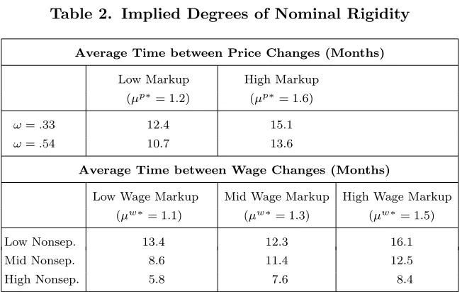
On the upper part of table 2, I report the implied degree of iner-tia (measured as the average time between price changes, measured in months) under two different assumptions about these two para-meters. For the parameter ω I consider two benchmark values, .33 and .54;37 for θ
p, which is related to the steady-state markup µ∗
by µ∗
= θp/(θp −1), I consider values that imply a low (20
per-cent) and a high (60 perper-cent) steady-state markup, two benchmark
37
As mentioned before, in the case of a Cobb-Douglas technology,ω=a/(1−a),
Table 2. Implied Degrees of Nominal Rigidity
Average Time between Price Changes (Months)
Low Markup High Markup (µp∗= 1.2) (µp∗= 1.6)
ω=.33 12.4 15.1 ω=.54 10.7 13.6
Average Time between Wage Changes (Months)
Low Wage Markup Mid Wage Markup High Wage Markup (µw∗= 1.1) (µw∗= 1.3) (µw∗= 1.5)
Low Nonsep. 13.4 12.3 16.1
Mid Nonsep. 8.6 11.4 12.5
High Nonsep. 5.8 7.6 8.4
values often used in the literature.38 As the table shows, the average duration of prices ranges from a little more than three quarters to about five quarters, depending on these assumptions.
The bottom part of the table shows the implied degree of wage inertia, computed in a similar manner. Here the inertia is summa-rized byγ= (1−αw)(1−βαw)
αw(1+θwχ) ; in order to make inference on αw,some
assumption must be made about the value of the parameters θw
and, therefore, about the value of the steady-state wage markup and about the degree of nonseparability between consumption and leisure in preferences, which determines the size of the parameterχ. In the table I consider different values for the steady-state markup and different degrees of nonseparability.39For low degrees of nonsep-arability, the average duration of wage contracts is similar to those of prices, while it is shorter for highly nonseparable preferences.
That preferences should be nonseparable in consumption and leisure is an implication of the negative sign of the elasticity of the
38
Values ofµ∗above 1.5 are, for example, estimated by Hall (1988) on a large
number of U.S. manufacturing industries.
39
marginal rate of substitution with respect to hours.40While most of the business-cycle literature adopts a separable preference specifica-tion, empirical evidence on significant nonseparability in preferences has been found, most recently, by Basu and Kimball (2000). More-over, within the class of preferences that are consistent with balanced growth, a negative elasticity of the marginal rate of substitution with respect to hours can be obtained in a generalized indivisible labor model, as shown in King and Rebelo (1999). The interpretation of the large elasticityηcis more problematic and requires further inves-tigation. As we will see below, however, a modification in the speci-fication of the time-series model reduces its size. Another possibility to be explored, which is left to future research, is that this para-meter is overestimated for an omitted variable problem in the wage equation, as would be the case if preferences were time dependent.
8. Some Robustness Analysis
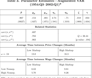
The inference presented on the structural parameters relies on the inference in the first step of the procedure: the estimation of the time-series model. I made a number of assumptions to model the VAR: the choice of variables was suggested by the need to limit its dimension, but the inclusion of additional variables could poten-tially improve the forecast of the driving forces of the structural equations. I modeled only one stochastic trend in the data, to mimic the trend assumption of the theoretical model; but the data may be consistent with other assumptions about the number of common stochastic trends. Finally, the VAR structure has been modeled as time invariant, while many recent analyses suggest that changes in policy regime have determined drifts over time in the reduced-form representation of the relation between nominal and real variables.41 While some of these issues are pursued in separate research,42 in table 3 I present the results of alternative estimates to shed
40
This can be shown by expressing the two elasticities of the marginal rate of substitutionηcandηhin terms of the Frish elasticities of consumption and labor supply (see Sbordone 2001).
41
See, for example, Boivin and Giannoni (2005) and Cogley and Sargent (2001, 2005).
42
Table 3. Parameter Estimates—Augmented VAR (1954:Q3–2002:Q1)*
β ̺p ̺w ηc ηh ζ γ
.967 .154 .001 2.74 –.71 .018 .033
.(0027) (.027) (.071) (.581) (.319) (.009) (.034)
Related Statistics
corr(π, πm) .897
corr(s, sm) .782 Q= 36.44
corr(ω, ωm) .903 [p-value: .194]
Average Time between Price Changes (Months)
Low Markup High Markup
ω=.54 13.0 16.3
Average Time between Wage Changes (Months)
Low Markup High Markup
Low Nonsep. 6.63 9.81
High Nonsep. 5.70 8.26
*The shorter sample is due to the federal funds rate data being available only from 1954:Q3.
some light on how sensitive the results presented so far are to the inclusion of additional variables in the time-series model. Specif-ically, I augment the baseline VAR with the federal funds rate: although the corresponding equation in the VAR is not meant to represent a policy rule, the introduction of the federal funds rate can be thought of as representing the reduced-form effect of mon-etary policy on inflation and the real variables of the system. The drawback of including an additional variable in the VAR, though, is an increase in uncertainty when the relative parameters are not tightly estimated.
9. Conclusion
In this paper I estimate the joint dynamics of U.S. prices and wages using a partial-information approach. I derive the implied price and wage inflations from an optimization-based model of staggered price and wage contracts with random duration and then implement a two-step minimum-distance estimation of the structural parameters. In the first step, I estimate an unrestricted time-series representa-tion for the variables of interest and derive the restricrepresenta-tions that the model solution imposes on this representation. In the second step, I use these restrictions to define a distance function to be minimized for the estimation of the structural parameters. This methodology allows me to investigate the dynamics of prices and wages without having to make all the additional assumptions required to close the model and to characterize its entire stochastic structure.
I find that a generalized version of the Calvo mechanism of ran-dom intervals between price and wage adjustments fits the data quite well, that there is some backward-looking component in inflation, and that the average duration of both contracts is around a year. The robustness of these results to the specification of the first stage of the proposed estimation procedure is to be further explored.
Appendix
Derivation of Equation (19)43
Under the hypothesis that there is a single stochastic trend driving long-run growth, say Θt, withγΘt = Θt/Θt−1 an i.i.d. process, one
can define stationary variables xwt ≡ XWwtt , πwt ≡ WWt−t1, ωt=
Wt
ΘtPt,
andvt= vt
Θt. Then, using the fact that
Xwt
Wt+j =
Xwt
Wt
Wt
Wt+j and
Xwt
Pt+j =
Xwt
Wt+j
Wt+j
Pt+j,equation (18) can be written as
Et
.
Σ∞
j=0(βαw)j
xwtΨwtjΠjk=1(πwt+k)
−1−θw
× Ht+j
xwtΨwtjωt+jΠjk=1(πtw+k)
−1− θw
θw−1
vt+j,t
/
= 0,
43
so that a log-linearization around steady-state valuesx∗ w, π
∗
, πw∗
, ω∗
, v∗
gives
Σ∞
j=0(βαw)j
ˆ
xwt+̺wΣj −1
k=0πˆt+k−Σjk=1πˆtw+k+ ˆωt+j
= Σ∞
j=0(βαw)j Et(ˆvt+j,t),
or
ˆ
xwt= (1−βαw)Σj∞=0(βαw)j Et
׈vt+j,t−ωˆt+j−̺wΣj −1
k=0πˆt+k+ Σjk=1πˆwt+k
. (49)
To express ˆvt+j,t in terms of the average marginal rate of
substitu-tion, I write
vt+j,t ≡
Λh
Λc(ct+j,t, ht+j,t) =
Λh
Λc(ct+j,t, ht+j,t)
Λh
Λc(ct+j, ht+j)
Λh
Λc(ct+j, ht+j)
,
(50)
where ct =Ct/Θt, and Λh denotes the marginal disutility of work.
Therefore, a log-linearization of (50) gives
ˆ
vt+j,t=ηc(ˆct+j,t−cˆt+j) +ηh(ˆht+j,t−ˆht+j) + ˆvt+j, (51)
where ηx (x = c, h) indicates the elasticity of the marginal rate
of substitution between leisure and consumption with respect tox, evaluated at the steady state. By the assumption that changes in consumption occur in a way that maintains the marginal utility of consumption equal across households, ˆct+j,t and ˆct+j are,
respec-tively, functions of ˆht+j,t and ˆht+j. Moreover, from (17) it follows
that
ˆ
ht+j,t−ˆht+j =−θw
ˆ
xwt+̺wΣj −1
k=0πˆt+k−Σjk=1πˆtw+k
.
Substituting this result in (51), I get
ˆ
vt+j,t=−χθw
ˆ
xwt+̺wΣj −1
k=0πˆt+k−Σ
j
k=1πˆwt+k
+ ˆvt+j, (52)
where I definedχ= −Λch
Λc
c ηc+ηh,and where Λ
c
i indicates the
In (15), dividing both sides byWt and log-linearizing, I obtain
ˆ
xwt=
αw
1−αw
(ˆπtw−̺wπˆt−1). (53)
Substituting (53) and (52) into (49), I obtain
(ˆπwt −̺wπˆt−1) =γΣ∞j=0(βαw)j Et
ˆ
vt+j−ωˆt+j
+ (1 +χθw)
Σjk=1πˆtw+k−̺wΣj −1
k=0πˆt+k , (54)
where γ= (1−αw)(1−βαw)
αw(1+θwχ) .
Finally, forwarding (54) one period, premultiplying it by βαw,
and subtracting the resulting expression from (54), I obtain the wage equation (19) in the text.
Empirical Implementation
To compute the solution, I cast the model in the following canonical form:
Yt+1=M Yt+ Ψut+1+ Πηyt+1, (55) where ηy,t+1=yt+1−Etyt+1 are expectational errors.
The definitions of the vector Yt and of the matrix M are as in
the text, and the matrices Ψ and Π are
Ψ =
⎡
⎣
N1 0
0 0
0 Q
⎤
⎦ and Π =
⎡ ⎣ 1 0 0 1 0 0 ⎤ ⎦. Furthermore,
Myy=
⎡ ⎢ ⎢ ⎢ ⎣
1+̺pβ
β − ζ
β − ̺p
β 0
̺w−̺p 1+β+βγ+ζ ̺p −̺w
β −
1
β
1 0 0 0
0 1 0 0
⎤ ⎥ ⎥ ⎥ ⎦,
MyZ =
⎡ ⎢ ⎢ ⎢ ⎣ 0
−γβΞ− 1
βe ′ q+e
As indicated in the text, the vector Ξ depends on the chosen speci-fication of preferences and on the assumptions about trend.
Sincevt=vT
t +vtcyc =qtT+vtcyc,from the definition of the trend
in productivity (47), it follows that
vt=qt+e′q[I−A]
−1A+η
cccyct +ηhhcyct ,
and the vector Ξ is therefore defined as
Ξ =e′
q[I−A]
−1A+η
c
e′ cy+e
′ h−e
′
q[I−A]
−1A+η
he′h
= (1−ηc)e′q[I−A]
−1A+η
c(e′cy+e ′
h) +ηhe′h
.
The parameters of interest in this expression are the elasticities ηc
andηh, which are estimated together with the adjustment parame-ters of the wage and price equations.
Inference on Wage Rigidity
To translate the estimate of the “inertia” parameterγ into an esti-mate of the degree of wage rigidity, I need to parameterizeχ,which is
χ= −Λ
c hH
Λc cC
ηc+ηh. (56)
I first consider a slight transformation of this expression:44
χ= −Λ
c hΛc
Λc cΛh
ΛhH
ΛcC
ηc+ηh (57)
and then write the expression forηc as
ηc =−
Λc cC
Λc +
Λc hC
Λh =σ+
Λc hC
Λh
=σ+Λ
c h
Λc c
ΛccC
Λc
Λc Λh =σ
1−Λ
c h Λc c Λc Λh , (58) 44
where, with conventional notation, I indicate with σ the inverse of the intertemporal elasticity of substitution in consumption. Expres-sion (58) implies that
Λc h
Λc c
Λc
Λh =
σ−ηc
σ ;
substituting this result in (57), I obtain
χ=
σ−ηc
σ ∗τ
ηc+ηh.
Therefore, given the estimated ηc and ηh, one can determine the
value of χ for any value that one wishes to assign to σ and to the ratio wH/C, which I have denoted by τ. The computations in table 2 are based on three different assumptions about the value of the intertemporal elasticity of substitution in consumption (corre-sponding toσ= 4,5, or 10) and the value ofτ = 1. Every value ofσ
implies, in turn, a different degree of nonseparability in preferences.
References
Altig, D., L. J. Christiano, M. Eichenbaum, and J. Lind´e. 2002. “Technology Shocks and Aggregate Fluctuations.” Unpublished. Amato, J. D., and T. Laubach. 2003. “Estimation and Control of an Optimization-Based Model with Sticky Prices and Wages.” Journal of Economic Dynamics and Control 27 (7): 1181–1215. Basu, S., and M. S. Kimball. 2000. “Long-Run Labor Supply and the Elasticity of Intertemporal Substitution for Consumption.” Unpublished, University of Michigan.
Batini, N., B. Jackson, and S. Nickell. 2005. “An Open-Economy New Keynesian Phillips Curve for the U.K.”Journal of Monetary Economics 52 (6): 1061–72.
Calvo, G. A. 1983. “Staggered Prices in a Utility-Maximizing Frame-work.”Journal of Monetary Economics 12 (3): 383–98.
Campbell, J. Y., and R. J. Shiller. 1987. “Cointegration and Tests of Present Value Models.” Journal of Political Economy 95 (5): 1062–88.
Christiano, L., M. Eichenbaum, and C. Evans. 2005. “Nominal Rigidities and the Dynamic Effects of a Shock to Monetary Pol-icy.” Journal of Political Economy 113 (1): 1–45.
Cogley, T., and T. J. Sargent. 2001. “Evolving Post-World War II U.S. Inflation Dynamics.” InNBER Macroeconomics Annual, ed. B. S. Bernanke and K. S. Rogoff, 331–73.
———. 2005. “Drifts and Volatilities: Monetary Policies and Out-comes in the Post WWII U.S.” Review of Economic Dynamics 8 (2): 262–302.
Cogley, T., and A. M. Sbordone. 2005. “A Search for a Structural Phillips Curve.” Staff Report No. 203, Federal Reserve Bank of New York.
Edge, R., T. Laubach, and J. Williams. 2003. “Productivity Slowdowns and Speedups: A Dynamic General Equilibrium Approach.” Unpublished, Board of Governors of the Federal Reserve System.
Erceg, C. J., D. W. Henderson, and A. T. Levin. 2000. “Optimal Monetary Policy with Staggered Wage and Price Contracts.” Journal of Monetary Economics 46 (2): 281–313.
Fuhrer, J., and G. Moore. 1995. “Inflation Persistence.” Quarterly Journal of Economics 110 (1): 127–59.
Gagnon, E., and H. Khan. 2005. “New Phillips Curve under Alter-native Technologies for Canada, the United States, and the Euro Area.” European Economic Review 49 (6): 1571–1602.
Gal´ı, J., and M. Gertler. 1999. “Inflation Dynamics: A Structural Econometric Analysis.”Journal of Monetary Economics 44 (2): 195–222.
Gal´ı, J., M. Gertler, and J. D. L´opez-Salido. 2001. “European Infla-tion Dynamics.” European Economic Review 45 (7): 1237–70. ———. 2005. “Robustness of the Estimates of the Hybrid New
Keynesian Phillips Curve.” Journal of Monetary Economics. 52 (6): 1107–18.
Hall, R. 1988. “The Relation Between Price and Marginal Cost in U.S. Industry.”Journal of Political Economy 96 (5): 921–47. Ireland, P. 1997. “A Small, Structural, Quarterly Model for
Mon-etary Policy Evaluation.”Carnegie-Rochester Conference Series on Public Policy 47:83–108.
King, R. J., and S. T. Rebelo. 1999. “Resuscitating Real Business Cycles.” In Handbook of Macroeconomics, Vol. 1B, ed. J. B. Taylor and M. Woodford, 927–1007. Elsevier Science.
Kurmann, A. 2005. “Quantifying the Uncertainty about the Fit of a New Keynesian Pricing Model.”Journal of Monetary Economics 52 (6): 1119–34.
Lind´e, J. 2005. “Estimating New-Keynesian Phillips Curves: A Full Information Maximum Likelihood Approach.”Journal of Mone-tary Economics 52 (6): 1135–49.
Rotemberg, J., and M. Woodford. 1997. “An Optimization-Based Econometric Framework for the Evaluation of Monetary Policy.” InNBER Macroeconomics Annual, ed. B. S. Bernanke and J. J. Rotemberg, 297–346.
Rudd, J., and K. Whelan. 2005. “New Tests of the New-Keynesian Phillips Curve.” Journal of Monetary Economics 52 (6): 1167–81.
Sbordone, A. M. 2001. “An Optimizing Model of U.S. Wage and Price Dynamics.” Working Paper Series 2001-10, Rutgers University.
———. 2002. “Prices and Unit Labor Costs: A New Test of Price Stickiness.” Journal of Monetary Economics 49 (2): 265–92. ———. 2005. “Do Expected Future Marginal Costs Drive Inflation
Dynamics?”Journal of Monetary Economics 52 (6): 1183–97. Sims, C. A. 2001. “Comments on Papers by Jordi Gal´ı and by
Stefania Albanesi, V.V. Chari and Lawrence J. Christiano.” Unpublished, Princeton University.
Smets, F., and R. Wouters. 2003. “An Estimated Dynamic Stochas-tic General Equilibrium Model of the Euro Area.”Journal of the European Economic Association 1 (5): 1123–75.
———. 2005. “Comparing Shocks and Frictions in US and Euro Area Business Cycles: A Bayesian DSGE Approach.”Journal of Applied Econometrics 20 (2): 161–83.
———. 1999. “Staggered Price and Wage Setting in Macroeconom-ics.” In Handbook of Macroeconomics, Vol. 1B, ed. J. B. Taylor and M. Woodford, 1009–50. Elsevier Science.