Performance Analysis of Image Segmentation Methods for the Detection of Masses in Mammograms

Performance Analysis of Image Segmentation Methods

for the Detection of Masses in Mammograms

Zainul Abdin Jaffery

Dept. of Electrical Engineering

Jamia Millia Islamia New Delhi, India

Zaheeruddin

Dept. of Electrical Engineering

Jamia Millia Islamia New Delhi, India

Laxman Singh

Dept. of Electrical Engineering

Jamia Millia Islamia New Delhi, India

ABSTRACT

Detection and quantification of breast cancer is a very critical step in mammograms and therefore, needs an accurate and standard technique for breast tumor segmentation. In the last four decades, a number of algorithms have been published in the literature. Each one has their own merits and demerits. The aim of this paper is to make a comparative analysis of the most promising methods, namely fuzzy c-means (FCM), k-means (KM), marker controlled watershed segmentation (MCWS) and region growing (RG), for the detection and segmentation of masses in mammographic images on real data obtained from Metro Hospital. Robustness of the methods is demonstrated by validating their quantitative results with expert manual data. It is observed that the RG gives better results compared to three other methods.

Keywords

Breast cancer, mathematical morphology, marker controlled watershed segmentation, region growing.

1.

INTRODUCTION

Cancer is one of the leading causes of human mortality in the world. The most common type of cancer in women is the breast cancer. Early detection and diagnosis leads to the successful treatment and thus play the key role in controlling the breast cancer deaths. Hence, it is essential for the women of age group 30-40 years to have regular screening every year. Currently, X-ray mammography is considered to be the most simple and reliable imaging method for the early detection of breast cancer [1]. Presence of masses or micro-calcification clusters on mammograms is considered to be preliminary indicators for early stage breast cancer. To determine the tumor area, in most of the hospitals, a radiologist performs the diagnosis of breast tumor manually on mammographic images. Visual examination of large volume of mammograms and shortage of experienced radiologists makes the process error prone and time consuming. Computer-aided diagnosis (CAD) system may help radiologist and doctors in reliable and precise diagnosis of breast cancer [2]. Numerous techniques have been developed and proposed as an emerging tool to segment masses from surrounding tissues in digital mammograms. Martins et al. [3] employed the K-means algorithm for mass detection on digitized mammograms and classified them into masses and non-masses through support vector machine using shape and texture descriptors. Dominguez et al. [4] applied three image segmentation methods, K-means, Fuzzy c-means and Possibilistic Fuzzy C-means, for the detection of microcalcification clusters and achieved the better segmentation results with Possibilistic Fuzzy C-means. Kannan et al. [5] proposed a kernel induced fuzzy c-means based hyper tangent function (KFCHF) algorithm for the segmentation of breast cancer from mammographic images. In this work, the objective function of standard fuzzy c-means was modified by replacing original

Euclidean distance on feature space using new hyper tangent function and the objective function thus obtained was converged more rapidly. Malek et al. [6] employed seed based region growing and mathematical morphology for the segmentation of microcalcifications in mammograms. Zaheeruddin et al. [7] presented the mean based region growing segmentation (MRGS) and marker controlled watershed segmentation (MCWS) for the segmentation of breast tumor in mammograms. Through the literature survey it is observed that each of the above mentioned algorithms or their modified versions have been used somewhere else but each method on different data sets.

Therefore, it is not possible to evaluate their performance directly without implementing all these four algorithms on common data sets. The region growing (RG) and marker controlled watershed segmentation (MCWS) are the region based methods and fuzzy C-means (FCM), K-means (KM) are clustering based methods. In the present work, four prominent methods for the image segmentation, namely, fuzzy C-means (FCM), K-means (KM), marker controlled watershed segmentation (MCWS), and region growing (RG) have been selected and an algorithm is developed for the detection of masses using these methods. This algorithm is tested using a number of mammographic images obtained from a diagnostic centre in New Delhi, India. The performance of these segmentation techniques are evaluated and analyzed.

2.

DETECTION METHODOLOGY

2.1

Image Enhancement

Geodesic dilation employs two input images namely, marker and mask images. Let h and g are two gray scale images defined on same domain such that h



g. Here, h is called the marker image and g is called the mask. Let

g

₁,

g

₂,

g

₃ ,………….,

g

_n be the connected components of g. The elementary geodic dilation of size 1 of the image h with respect to a reference image g is given by [9]

P

g

(

h

)



(

h



b

)



g

;

h



g

) 1 (

(1)

where,



is the point-wise minimum and

_P

(1)

(

_h

)

g is

defined as the minimum between h dilated by a structuring element b and g. Similarly the elementary geodic erosion of size 1 of the image h (marker image) with respect to a reference image g (mask image) is given by

E

(

h

)

(

h

) 1 (

g



Ө

b

)



g

(2)

where,



is the point-wise maximum and

_E

(1)

(

_h

)

g is

defined as the maximum between h dilated by a structuring element b and g. The geodesic dilation and erosion of size n is obtained as:

P

(

h

)

P

(

P

(

h

))

) 1 n ( g ) 1 ( g ) n ( g 



(3)

(

)

(

(

))

) 1 ( ) 1 ( ) (

h

E

E

h

E

_gn



_{g g}n (4) The desired morphological reconstruction is obtained when

)

(

) (

h

P

_gn =

P

_g(n1)

(

h

)

and,

E

_g(n)

(

h

)

=

E

_g(n1)

(

h

)

, that means, until condition of stability is reached. Thus, reconstruction by dilation is denoted as

R

_gD

(

h

)

, i.e.,

)

(

)

(

h

P

( )

h

R

_gD



_gn , if

P

_g(n)

(

h

)



P

_g(n1)

(

h

)

(5)

Similarly, reconstruction by erosion denoted as

R

_gE

(

h

)

is

)

(

)

(

h

E

( )

h

R

_gE



_gn , if

E

_g(n)

(

h

)



E

_g(n1)

(

h

)

(6) On the basis of these operations, opening by reconstruction is defined as

O (h) R (h

D h )

n (

R  Ө

nb

)

₍₇₎

Similarly, closing by reconstruction is defined as

C

h

R

h

E h n

R

(

)

(

)

(





)

nb

(8)

2.2 Segmentation Methods

A number of segmentation methods have been proposed by the researchers in the literature to extract the region of interest from image. Following segmentation algorithms have been considered here for their performance analysis.

2.2.1. Fuzzy c-means (FCM) algorithm

FCM is the unsupervised pixel classification technique that aims at dividing image pixels into optimal number of clusters. It was first proposed by Dunn et al. [11]. In general, pixels in

a cluster have high degree of similarity than those in different clusters. However, each pixels of image possesses certain degree of similarity with the pixels of every cluster. This degree of belonginess is represented by a fuzzy membership function. The FCM algorithm assigns each pixel to more than one cluster with different membership degrees.

Let X = (x1, x2,...,xN) represents an image with N pixels to be

divided into c clusters, where xi denotes a multispectral data,

then the clusters are formed by the iterative optimization of the following objective function [12 ].

Jp =





 

c

i N

j 1 1

u_ijp

x

_j



v

_i 2

(9)

where, uij is the fuzzy membership degree of pixel xjin the

cluster i, vi is the cluster center of ith cluster, and p is a

constant that controls the fuzziness of the resulting partitions. No theoretical basis exists for the selection of optimal value of p; usually its value is chosen to be 2. The FCM objective function is minimized when pixels in the proximity of cluster centroids are assigned high membership values, and low membership values are assigned to pixels far from the centroid of corresponding clusters. The membership grade matrix U is created for all pixels and clusters. The FCM algorithm can be described as follows:

1. Initialize the membership matrix U = [uij]1ic,1 j N

in the range [0,1] such that the element of uij of U satisfies the

criteria



 c i ij

u

1

=1,j=1,2,…,N (10)

2. Compute the center vi of their respective fuzzy clusters

using

vi=





  N j p ij N j j p ij

u

x

u

1 1 (11)

3. Update the membership functions using

uij =



 





















c L p L j i j

v

x

v

x

1 ) 1 /( 2

1

(12)

4. Repeat step 2 and 3 until the iteration convergence criterion is satisfied,

maxij



u

_ijq1



u

_ijq



<



,

(13)

converge to a local minimum or a saddle point of objective function Jp.

2.2.2 K-means (KM) algorithm

K-means is known as one of the simplest unsupervised learning algorithms that are used to partition an image into K

-clusters [4]. It is an iterative technique which follows a simple procedure to classify a given data set, W, in d-dimensional space, through a K-number of clusters (which are fixed a priori). The first step intends to define a single prototype for each cluster (K-prototypes for K-clusters). In the next step, each data point is associated to the cluster with the nearest prototype. These prototypes must be placed in a cunning way with a distance as maximum as possible to yield a different results. The space partition of input data is updated and then new values of K-prototypes are re-calculated every time a pixel (data point) is added to the cluster. The algorithm is iterated until no data point is exchanged between clusters. The objective of this algorithm is to minimize the objective function that represents the total intra-cluster variance. This objective function is given as [4]:

2

1 1 ) (



 





c

j n

i

j j

i

z

w

J

, (14)

where,

2 j ) j ( i z

w  is distance measure between every data point,

w

_i(j), and the cluster center,

z

_j. The objective function indicates the similarity between n data points (pixels) and their cluster prototypes. The algorithm is described by the following steps.

1) Select appropriate number of K-points as initial prototypes to initiate the algorithm.

2) Construct a new partition by assigning each data point to the nearest prototype.

3) Re-calculate the new values of K-prototypes by taking the average value of all the points linked with the cluster. 4) Repeat steps 2 and 3 until the positions of the cluster

prototypes no longer change. The result is that all the data points are grouped into final required number of clusters.

2.2.3 Marker controlled watershed (MCWS)

segmentation

Watershed algorithm is considered as a powerful tool for image segmentation. It plays an important role in machine vision, video image segmentation and image analysis [13]. Basic idea of watershed algorithm is to view the gradient of gray scale image as a topographic surface, wherein the rain falling on the watershed line would be collected equally in catchments basins. The line that separates two catchment’s basins is referred as watershed line as shown in Fig. 1. Vincent and Soille [14] proposed the novel approach for finding the watershed lines by using the immersion simulation algorithm. Segmentation efficacy of the watershed transform is improved significantly, if foreground objects and background regions are marked already.

In order to compute the gradient magnitude image, linear filtering operations such as average filtering and simple arithmetic calculations are used. However, if watershed algorithm is directly applied on gradient magnitude image,

there always occurs an over segmentation mainly due to the presence of large number of minima’s in that image. Therefore, markers of desired size are computed before applying watershed transform on gradient magnitude image. The catchment basins possessing minimal value are not marked properly in the presence of noise. Hence, before applying the watershed algorithm, pre-processing step is employed to remove the noise and other kind of non-uniformity from the test image in order to mark only the desired catchment basins. These marked catchment basins produce the modified gradient image. Watershed transform is then applied on modified gradient image to yield the final watershed ridge lines. The resultant image is finally superimposed on the original image to display the overall segmentation result.

Fig1: Watershed lines with catchments basins.

2.2.4. Region growing (RG) algorithm

In image segmentation, a region that corresponds to an object is defined as the group of spatially connected pixels having some property in common (such as similar gray levels) [15]. Region growing method relies on the propagation of an initial seed point according to pre-defined homogeneity criterion [16]. All neighboring pixels that have similar properties as that of seed pixel are appended to it, thus iteratively increases the size of region. A neighboring pixel is said to be similar to seed pixel if it satisfies the homogeneity criterion. At each iteration, all those pixels that reside near the boundary of growing regions are examined. If the pixel is found to be most similar to a region based on the given criterion, then it gets added to that region. This process continues until all the pixels get assimilated [17]. If the gray level value of the neighboring pixel is within deviation range of given threshold, then, it is labeled as foreground otherwise as a background pixel. In this method, appropriate values of seed pixel (Sf) and threshold (T)

are computed automatically using the Equation (15) and (16) respectively [7].

Sf =

N

M



1

_

_

  



1

0 1

0

)

,

(

M

y N

x

y

x

f

(15)

T =

4

)}

,

(

{

f

x

y

Entropy

S







(16)

The value of



depend upon the variability in the intensities of foreground and background. Here, its value is assumed between 0 and 1. Above found values of seed pixel and threshold are used in basic region growing method for accurate and fast segmentation of abnormal regions in mammogram. The above equations give the approximate values of seed pixel and threshold which can easily be fine tuned to obtain the desired results. Region growing algorithm yields better results segmenting only highly homogenous regions, if the seed pixel and threshold values are chosen accurately.

3. IMPLEMENTATION

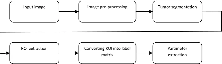
The process flow diagram for the detection of the tumor region using the segmentation methods, as discussed above, is shown in fig. 2. The proposed algorithms are simulated on MATLAB 7.0 on a personal computer with a processor speed of 1.8 GHz and 2GB memory. About 18 mammogram images are procured from a diagnostic centre of Metro hospital, Faridabad, NCR of New Delhi. Each mammogram was pre-processed with opening-closing morphological filtering technique. Structuring elements of different sizes were used to filter out the noise and other artifacts in mammograms. The pre-processing of one sample image is shown in fig. 3. After pre-processing, each image is segmented using image segmentation algorithms discussed in section 2.

4. REGION OF INTEREST (ROI)

SELECTION

In this work, after segmentation of region of interest, we compute area of all the tumors extracted by each method. To proceed towards area measurement, we first separate out ROI from the segmented image. Thereafter, separated ROI is converted into label matrix. Area of extracted region is then computed and compared with the area furnished by an expert radiologist. The segmentation result for one set of image using above segmentation methods are shown in fig.4. After segmentation, the ROI is extracted and is shown in fig.5.

5. RESULTS AND DISCUSSION

The simulation is done for a number of images and the tumor area is computed for each images. The results obtained from simulation are tabulated in table1. The relative error (RE) of each method for different tumor area is computed as:

RE (%) =

_









 

' '

A

A

A

_

100 (17)

where

A

is the tumor area measured by different approaches and

A

' represents the tumor area as furnished by an expert radiologist. The comparison of relative errors using FCM, KM, MCWS, and RG methods are given in table 2. After

applying each algorithm one by one on all mammographic images, following statistics parameters are evaluated for further analysis [18]:

(i) Sensitivity = Detected true positives / Real number of positives.

(ii) Number of false positive per image = Total number of false alarms / Total number of images.

Tumor area with relative error less than 50 percent is considered as detected ‘true positives’, otherwise as ‘false positives’. Therefore, in true sense, sensitivity presents the tumor detection rate for each method considering only those tumors whose segmented area matches at least 50 percent of the area furnished by the expert radiologist. All the segmented objects other than tumor are also considered as false alarms. Table 3 gives sensitivity, number of false positives per images and the relative error. Segmentation results are rated in one of the five possible labels: VG ― very good (with relative error range, 0-10%), G ― good (with relative error range, 11-20%), AVG ― average (with relative error range, 21-30%), BAVG

― below average (with relative error range, 31- 42%), B ―

bad (with relative error range, >42%). From the table3, it is observed that, RG method yielded better results compared to other methods, with 72.20% of segmented masses rated very good (VG). Its score was one (B = 1) for bad cases. However, KM method achieved worst score with 4 bad cases, and 7 very good cases. Number of bad cases (B = 4), and very good cases (VG = 12), both were high in case of FCM method. MCWS got the average score with 3 bad cases, and 10 very good cases. From the above discussion, it can be said that RG method segmented the tumors more accurately than the others with the least deviation from the actual one (outlined by an expert radiologist) in maximum number of cases (VG = 13). After RG method, FCM method achieved the higher segmentation accuracy of the extracted tumors with 12 very good cases. . The FCM achieved the sensitivity of 77.80% with 2.50 false positives per image, KM with sensitivity of 77.80% at the rate of 3.92 per image, MCWS with sensitivity of 83.30% at the rate of 3.50 per image, and with sensitivity of 94.44% at the rate of 1.12 per image by RG method. Thus, RG method seems to provide good segmentation results with 94.44% sensitivity at the rate of 1.12 FP/image, and with maximum number of cases segmented with greater accuracy than any other method presented here.

6. CONCLUSION

[image:5.595.102.491.71.183.2]

Fig 2: Flow diagram for the detection of tumor

(a) (b) (c) (d)

Fig3: Image enhancement by morphological open–close reconstruction filter with structuring elements of different window size, (a) Original sample mammograms, (b) image enhancement with window size 3×3, (c) image enhancement with window size 5×5, (d) image enhancement with window size 7×7 .

and accuracy limitations of the available methods. But, the major drawback of this method is its dependence on appropriate selection of threshold and seed pixel value which makes it more time consuming and complicated. But another point of view that makes it more useful is that the less accurate methods are considered similar to non-interactive

methods in the domain of medical image analysis, and therefore pose hindrance to their widespread use in clinics. The collective efforts of radiologists and the proposed method as a pre-reader would result in accurate diagnosis. The quantitative evaluation of the segmentation results for FCM, KM, MCWS, and RG methods are summarized in Table 3.

(a) (b) (c) (d) (e)

Fig4: Segmentation results: (a) Original sample mammogram, (b) using FCM, (c) using KM, (d) using MCWS, (e) using Region growing (RG).

(a) (b) (c) (d)

Fig5: Extracted tumor area (a) using FCM method, (b) using KM method, (c) using MCWS method, (d) using RG method.

Input image Image pre-processing Tumor segmentation

ROI extraction Converting ROI into label matrix

[image:6.595.114.483.95.418.2]

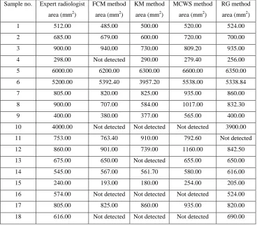
Table 1. Comparison of various methods with expert radiologist data for different tumor area

Table 2. Comparison of relative errors for different tumor area.

Sample no. Expert radiologist area (mm2)

FCM method area (mm2)

KM method area (mm2)

MCWS method area (mm2)

RG method area (mm2)

1 512.00 485.00 500.00 520.00 524.00

2 685.00 679.00 600.00 720.00 700.00

3 900.00 940.00 730.00 809.20 935.00

4 298.00 Not detected 290.00 279.40 256.00

5 6000.00 6200.00 6300.00 6600.00 6350.00

6 5200.00 5392.40 3957.20 5538.00 5338.84

7 805.00 820.00 825.00 935.00 860.00

8 900.00 707.00 584.00 1017.00 832.30

9 400.00 380.00 377.00 565.00 400.00

10 4000.00 Not detected Not detected Not detected 3900.00

11 753.00 763.40 910.00 792.60 Not detected

12 860.00 901.00 739.00 1160.00 842.50

13 675.00 650.00 Not detected 655.00 650.00

14 545.00 567.00 561.70 580.00 616.00

15 240.00 193.00 180.00 254.00 205.00

16 574.00 Not detected Not detected Not detected 524.00

17 805.00 825.00 860.00 935.00 820.00

18 616.00 Not detected Not detected Not detected 690.00

Sample no. Relative error (%) FCM

Relative error (%) KM

Relative error (%) MCWS

Relative error (%) RG

1 5.30 3.50 1.60 1.14

2 0.87 12.40 5.10 2.20

3 4.40 18.90 10.10 3.90

4 - 2.70 6.20 11.70

5 3.30 5.00 10.00 5.80

6 3.70 23.90 6.50 2.67

7 1.86 2.50 16.1 6.80

8 21.40 35.10 13.00 7.52

9 5.00 5.75 41.30 0.00

10 - - - 2.50

11 1.38 20.80 5.30 -

12 4.77 14.10 34.80 2.03

13 3.70 - 2.96 3.70

14 4.04 3.06 6.42 13.03

15 19.60 25.00 5.83 14.60

16 - - - 8.70

17 2.48 6.83 16.10 1.86

Table3. Comparative analysis of algorithms using statistical data.

REFERENCES

[1] Cheng, H. D., Shi, X. J., Min, R., Hu, L. M., Cai, X. P., and Du, H. N. 2006. Approaches for automated detection and classification of masses in mammograms. Pattern Recog. 39, 646-668.

[2] Oliver, A., Freixenet, J., Marti, J., Perez, E., Pont, J., Denton, E., and Zwiggelaar, R. 2010. A review of automatic mass detection and segmentation in mammographic images. Medical Image Analysis. 14, 87-110.

[3] Martins, L., Junior, G. B., Silva, A. C., Paiva, A. C., and Gattass, M. 2009. Detection of Masses in Digital Mammograms using K-means and Support Vector Machine. Electronic Letters on computer Vision and Image Analysis. 8, 39-50.

[4] Dominquez, J. Q., Magana, B. O., Januchs, M. G., Ruelas, R., Corona, A. V., Andina, D. 2011. Image segmentation by fuzzy and possibilitic clustering algorithms for the identification of microcalcifications. Scientia Iranica D. 18, 580 – 589.

[5] Kannan, S. R., Ramathilagam, S., Devi, R., Sathya, A. 2011. Robust kernel FCM in segmentation of breast medical images. Expert Systems with Applications. 38, 4382-4389.

[6] Malek, A., Rahman, W. A., Ibrahim, A., Mahmud, R., Yasiran, S. S. 2010. Region and boundary segmentation of microcalcification using seed based region growing and mathematical morphology. In Proc. Int. Conference on Mathematics Education Research. 8, 634-639. [7] Zaheeruddin, Jaffery, Z. A., and Singh, L. 2012.

Detection and shape feature extraction of breast tumor in mammograms. In Proc. World Congress on. Engineering 2012. Vol. II (London, U.K).

[8] Gonzalez, R. C., and woods, R. E. Digital Image Processing. 2nd _{Ed. New Delhi: Pearson Education.}

[9] Vincent L 1993. Morphological grayscale reconstruction in image analysis: applications and efficient algorithms. IEEE Trans. Image Processing. 2, 176-201.

[10]Mukhopadhyay, S., Chanda, B. 2003. Multiscale morphological segmentation of gray-scale images. IEEE Trans. Image Processing. 12, 533-548.

[11]Dunn, J. 1974. A fuzzy relative of the ISODATA process and its use in detecting compact well separated clusters. J. cybernetics. 3, 32-57.

[12]Tan, K. S., Isa, N. A. 2011. Color image segmentationm using histogram thresholding – fuzzy c-means hybrid approach. Pattern Recog. 44, 1-15.

[13]Lin, Y. C., Tsai, Y. P., Hung, Y. P., Shih, Z. C. 2006, Comparison between immersion-based and toboggan– based watershed image segmentation. IEEE Trans. Image Processing. 15, 632-640.

[14]Vincent, L., Soille, P. 1991. Watersheds in digital spaces: an efficient algorithm based on immersion simulations. IEEE Trans. Pattern and Machine Intelligence. 13, 583-598.

[15]Shen, L., Rangayyan, R. M., Desautls, J. L. 1994. Aplication of shape analysis to mammographic calcifications. IEEE Trans. Medical Imaging. 13, 263-274.

[16]Adams, R., and Bischof, L. 1994. Seeded region growing. IEEE Trans. Pattern and Machine Intelligence. 16(6), 641-647.

[17]Mehnert, A., Jackway, A. 1997. An improved seeded region growing algorithm. Pattern Recognition Letters. 18, 1065-1071.

[18]Zheng L, Chan A. K. 2001. An artificial intelligent algorithm for tumor detection in screening Mammogram. IEEE Trans. Medical Imaging. 20, 559-567.

Recognition Statistics

FCM KM MCWS RG Relative Error

Range (%)

VG 12 07 10 13 0-10

G 01 04 03 04 11-20

AVG 01 02 Nil Nil 21-30

BAVG Nil 01 02 Nil 31-42

B 04 04 03 01 > 42

VG (%) 66.70 38.90 55.60 72.20

Sensitivity (%) 77.80 77.80 83.30 94.44