A New Approach for Dynamic Time Quantum Allocation
in Round Robin Process Scheduling Algorithm
Ritika Gakher
,Department of Computer Science, FMIT Jamia Hamdard, New Delhi
Saman Rasool,
Department of Computer Science, FMIT Jamia Hamdard, New Delhi
ABSTRACT
Round-Robin (RR) is the vastly used process scheduling algorithm where, all processes are allocated some time shares in a circular order. If a process is able to complete its execution within this time quantum share, it is removed from the ready queue else it goes back at the end of the queue. Round-Robin scheduling is simple, gives fair allocation of CPU to the process and is starvation free. However there is few performance issues related to it. One of them is that even if there is a fractional amount of time left for a process to complete it execution, and its time share expires, it is preempted. Now this process has to wait unnecessarily to get its next chance to complete this fractional remaining execution. In this paper the proposal for the modification which will eradicate this performance issue of the conventional round robin algorithm is proposed thereby making it fairer.
Keywords
Time Quantum, Turnaround Time, Number of Cycles, Remaining Time, Number of Context switches, Wait time
.
1.
INTRODUCTION
An operating system may be defined as the interface between the user and the hardware.[1][2] Among numerous functionalities of the operating system, the most essential one is the job of process scheduling in which the operating system chooses which process will be executed first and in what manner.[3][4][6]
Benchmark of a good scheduling algorithm depends on the following criteria:
All processes should get equal share at the central processing unit.
CPU should be at work all the time i.e. it should not be idle.
Response time should be minimized.
Numbers of jobs executed per unit time should be maximized
There are several scheduling algorithms available some of them include:
1.1
First Come First Serve (FCFS)
In this algorithm, the process that reaches first at the CPU will be executed first. The CPU will be accessible to the process until the time the process completes its execution or performs an I/O operations.[1][10][11].
1.2
Shortest Job First (SJF)
In this algorithm the process that has the shortest burst time will be executed first by the CPU, then the process with the next higher burst time will be executed and so on. Here also the CPU will be available to the process until the time the process completes its execution or performs an I/O operation [3][4][7][10]
1.3
Round Robin (RR)
The viewpoint of this algorithm is similar to that of FCFS except the fact that the process will be executed by the CPU for a fixed time quantum. If the process gets completed within this period, it is removed from the ready queue otherwise it goes back at the end of the ready queue and waits for its next chance.[1][3][5]
1.4
Priority Scheduling
In this algorithm, the process with the highest priority is arranged first thereby executed first by the CPU. [6][7]
1.5
Multilevel queue scheduling
In this the ready queue is segregated into a number of different queues. The assignment of the processes to one of the queue permanently is usually based on properties of the processes such as memory size, process priority of type of process.[3][10][11]
1.6
Multilevel feedback queue scheduling
This algorithm is similar to the multilevel queue scheduling but it permits process to move between the queues.[9][10][11]
1.7
Lottery scheduling
The basic idea of this kind of scheduling is that the CPU gives the processes lottery tickets for provision of CPU time. A lottery ticket is chosen at random at the time of scheduling decision and the process holding the ticket gets the CPU.[1][2][8]
2.
RELATED WORKS
the result by 80 percentages. In [6], the researchers, recommended an algorithm namely, fuzzy round robin algorithm that tried to remove the problem with the CPU round robin scheduling that is, if the time requisite for the running process is some extent more than time quantum even by a fraction value, then the process gets forestalled and context switch occurs. This algorithm also eliminated the problem with the time quantum of RR scheduling, that is if it is too large, the algorithm degenerates to FCFS or it worsens the performance otherwise. The authors in [7], made slight changes to the conventional round robin algorithm where the time quantum of the scheduled processes is augmented to some amount whose remaining time in its last turn is less than or equal to a given threshold value, which is one–fourth of the time quantum. In [8], the novelists talked about dynamic quantum precision wherein a processor is said to be optimally implemented if it has highest throughput, low wait time, low turnaround time and less no of context switches for process coming to execution. This proposal worked by finding the left out B.T. of processes in the last but one turn of each processed to get an optimal threshold value also the processes has been divided into two categories, first category modifies time quantum and second will be processed as per classical RR algorithm. The researchers of [9] followed a mathematical approach which attempts to mathematically formularize the computation of waiting time of any process in a static n processes, CPU bound a round robin scheme which also calculated other performance measures as well. The approach followed uses two ready queue, wherein a process is returned to second ready queue after completion of last round. This reduces average waiting time and increases throughput while level of C.P.U utilization is preserved and there is no substantial increase in overheads.
3.
PROPOSED APPROACH
For each process, the square root of the burst time is inferred. In the proposed approach the time quantum is modified for the process which requires a fractional more time than allocated time quantum cycle(s) using the threshold value ‘K’ which is calculated as
K =
(TQ-
SQ/N)
SQ= sqrt (BT [Pi])The other parameters are calculated as follows NOC [Pi] =
(BT
[Pi]/TQ)
RT [Pi] = BT[Pi] % TQ
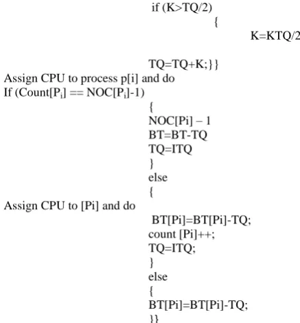
The pseudo code given below presents the proposed approach ImpRoundRobin(TQ, BT[i])
{
count[Pi] = 1; ITQ = TQ; if (BT[i]<=TQ) assign the CPU to process P[i]
else
if (BT[Pi]%TQ==0) {
assign CPU to the process P[i] and do
BT[Pi]=BT[Pi]-TQ; count[Pi]++; }
else if (BT[Pi]%TQ!=0) { else if (RT<=K) {
if (K<=TQ/2) {
TQ=TQ+K;}}
if (K>TQ/2) {
K=KTQ/2;
TQ=TQ+K;}} Assign CPU to process p[i] and do If (Count[Pi] == NOC[Pi]-1)
{
NOC[Pi] – 1 BT=BT-TQ TQ=ITQ } else { Assign CPU to [Pi] and do
BT[Pi]=BT[Pi]-TQ; count [Pi]++; TQ=ITQ; } else {
BT[Pi]=BT[Pi]-TQ; }}
Table 1(a): Table of processes for example 1 using conventional round robin
Process Name Burst Time (BT)
P1 15
P2 16
P3 25
P4 18
P5 31
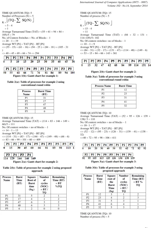
TIME QUANTUM (TQ): 5
Average Turnaround Time (TAT) = (55 + 76 + 94 + 84 + 105)/5 = 82
No. of Context Switches = No. of Blocks – 1 => 23 – 1 = 22
Average WT [Pi] = TAT [Pi] – BT [Pi]
=> (55 – 15) + (76 – 16) + (94 – 25 ) + (84 – 18 ) + (105 – 31 )
=> 40 + 60 + 69 + 66 + 74 => 309
Figure 1(a): Gantt chart for example 1
Table 1(b): Table of processes for example 1 using proposed approach
Process Name
Burst Time (BT)
Square Root of the Burst Time (Sq.)
Number of cycles (NOC) = BT / TQ
Remaining Time (RT) = BT %
TQ
P1 15 3 3 0
P2 16 4 3 1
P3 25 5 5 0
P4 18 4 3 3
[image:2.595.302.553.66.686.2] [image:2.595.313.532.72.308.2]TIME QUANTUM (TQ): 5 Number of Processes (N) = 5
K =
(TQ
-
SQ/N)
= 5 – 4= 1
Average Turnaround Time (TAT) = (55 + 61 + 94 + 84 + 105)/5 = 79
No. of Context Switches = No. of Blocks – 1 => 20 – 1 = 19
Average WT [Pi] = TAT [Pi] – BT [Pi]
=> (55 – 15) + (61 – 16) + (94 – 25 ) + (84 – 18 ) + (105 – 31 )
=> 40 + 45 + 69 + 66 + 74 => 294
Figure 1(b): Gantt chart for example 1:
Table 2(a): Table of processes for example 2 using conventional round robin
Process Name
Burst Time (BT)
P1 31
P2 17
P3 47
P4 48
P5 6
TIME QUANTUM (TQ): 15
Average Turnaround Time (TAT) = (114 + 83 + 146 + 149 + 66)/5 = 111
No. Of context switches = no of blocks – 1 => 14 – 1 = 13
Average WT [Pi] = TAT [Pi] – BT [Pi]
=> (114 – 31) + (83 – 17) + (146 – 47) + (149 – 48) + (66 – 6) => 83 + 66 + 99 + 101 + 60 => 409
Figure 2(a): Gantt chart for example 2:
Table 2(b): Table of processes for example 2 using proposed approach
Process Name
Burst Time (BT)
Square Root of Burst
time (Sq.)
Number of cycles (NOC) = BT / TQ
Remaining Time (RT)
= BT %TQ
P1 31 5 2 1
P2 17 4 1 2
P3 47 6 3 2
P4 48 6 3 3
P5 6 2 0 0
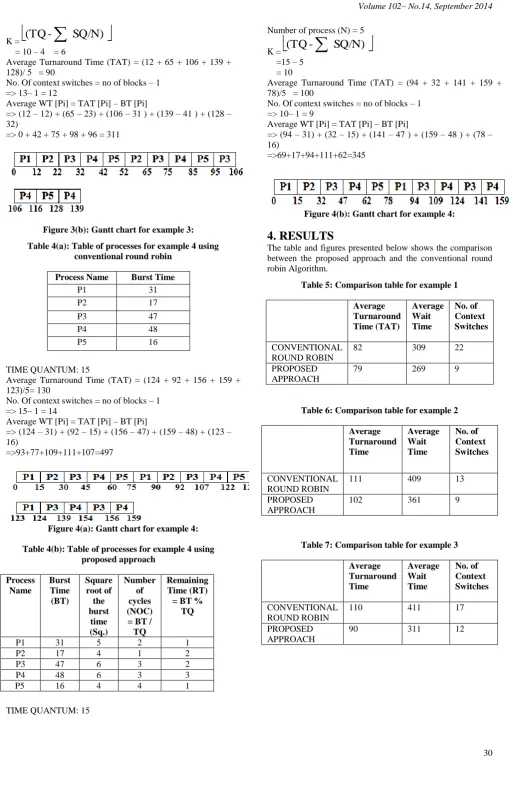
TIME QUANTUM (TQ): 15
Number of process (N) = 5
-
K =
(TQ
-
SQ/N)
= 15 – 4= 11
Average Turnaround Time (TAT) = (84 + 32 + 131 + 114+149)/5= 102
No. Of context switches= no of blocks – 1 => 10 – 1 = 9
Average WT [Pi] = TAT [Pi] – BT [Pi]
=> (84 – 31) + (32 – 17) + (131 – 47) + (114 – 48) + (149 – 6) => 53 + 15 + 84 + 66 + 143 = 361
Figure 2(b): Gantt chart for example 2:
Table 3(a): Table of processes for example 3 using conventional round robin
Process Name Burst Time
P1 12
P2 23
P3 31
P4 41
P5 32
TIME QUANTUM (TQ): 10
Average Turnaround Time (TAT) = (52 + 95 + 126 + 139 + 138)/ 5 = 110
No. Of context switches = no of blocks – 1 => 18– 1 = 17
Average WT [Pi] = TAT [Pi] – BT [Pi]
=> (52 – 12) + (95 – 23) + (126 – 31) + (139 – 41) + (138 – 32)
=>40 + 72 + 95 + 98 + 106 = 411
Figure 3(a): Gantt chart for example 3:
Table 3(b): Table of processes for example 3 using proposed approach
Process Name
Burst Time (BT)
Square root of the Burst Time (Sq)
Number of cycles (NOC) = BT / TQ
Remaining Time (RT) = BT %
TQ
P1 12 3 1 2
P2 23 4 2 3
P3 31 5 3 1
P4 41 6 4 1
P5 32 5 3 2
[image:3.595.47.553.34.799.2]K =
(TQ
-
SQ/N)
= 10 – 4 = 6Average Turnaround Time (TAT) = (12 + 65 + 106 + 139 + 128)/ 5 = 90
No. Of context switches = no of blocks – 1 => 13– 1 = 12
Average WT [Pi] = TAT [Pi] – BT [Pi]
=> (12 – 12) + (65 – 23) + (106 – 31 ) + (139 – 41 ) + (128 – 32)
=> 0 + 42 + 75 + 98 + 96 = 311
Figure 3(b): Gantt chart for example 3:
Table 4(a): Table of processes for example 4 using conventional round robin
Process Name Burst Time
P1 31
P2 17
P3 47
P4 48
P5 16
TIME QUANTUM: 15
Average Turnaround Time (TAT) = (124 + 92 + 156 + 159 + 123)/5= 130
No. Of context switches = no of blocks – 1 => 15– 1 = 14
Average WT [Pi] = TAT [Pi] – BT [Pi]
=> (124 – 31) + (92 – 15) + (156 – 47) + (159 – 48) + (123 – 16)
=>93+77+109+111+107=497
Figure 4(a): Gantt chart for example 4:
Table 4(b): Table of processes for example 4 using proposed approach
Process Name
Burst Time (BT)
Square root of the burst
time (Sq.)
Number of cycles (NOC) = BT / TQ
Remaining Time (RT) = BT %
TQ
P1 31 5 2 1
P2 17 4 1 2
P3 47 6 3 2
P4 48 6 3 3
P5 16 4 4 1
TIME QUANTUM: 15
Number of process (N) = 5
K =
(TQ
-
SQ/N)
=15 – 5= 10
Average Turnaround Time (TAT) = (94 + 32 + 141 + 159 + 78)/5 = 100
No. Of context switches = no of blocks – 1 => 10– 1 = 9
Average WT [Pi] = TAT [Pi] – BT [Pi]
=> (94 – 31) + (32 – 15) + (141 – 47 ) + (159 – 48 ) + (78 – 16)
=>69+17+94+111+62=345
Figure 4(b): Gantt chart for example 4:
4. RESULTS
The table and figures presented below shows the comparison between the proposed approach and the conventional round robin Algorithm.
Table 5: Comparison table for example 1
Average Turnaround Time (TAT)
Average Wait Time
No. of Context Switches
CONVENTIONAL ROUND ROBIN
82 309 22
PROPOSED APPROACH
79 269 9
Table 6: Comparison table for example 2
Average Turnaround Time
Average Wait Time
No. of Context Switches
CONVENTIONAL ROUND ROBIN
111 409 13
PROPOSED APPROACH
[image:4.595.48.562.47.833.2]102 361 9
Table 7: Comparison table for example 3
Average Turnaround Time
Average Wait Time
No. of Context Switches
CONVENTIONAL ROUND ROBIN
110 411 17
PROPOSED APPROACH
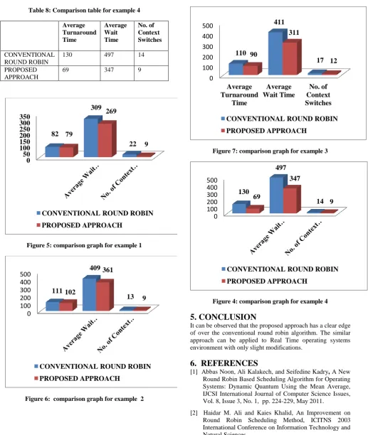
Table 8: Comparison table for example 4
Average Turnaround Time
Average Wait Time
No. of Context Switches
CONVENTIONAL ROUND ROBIN
130 497 14
PROPOSED APPROACH
69 347 9
[image:5.595.48.566.63.676.2]Figure 5: comparison graph for example 1
Figure 6: comparison graph for example 2
Figure 7: comparison graph for example 3
Figure 4: comparison graph for example 4
5. CONCLUSION
It can be observed that the proposed approach has a clear edge of over the conventional round robin algorithm. The similar approach can be applied to Real Time operating systems environment with only slight modifications.
6. REFERENCES
[1] Abbas Noon, Ali Kalakech, and Seifedine Kadry, A New Round Robin Based Scheduling Algorithm for Operating Systems: Dynamic Quantum Using the Mean Average, IJCSI International Journal of Computer Science Issues, Vol. 8, Issue 3, No. 1, pp. 224-229, May 2011.
[2] Haidar M. Ali and Kaies Khalid, An Improvement on Round Robin Scheduling Method, ICITNS 2003 International Conference on Information Technology and Natural Sciences.
[3] Shanmugam Arumugam and Shanthi Govindaswamy, Performance of the Modified Round Robin Scheduling Algorithm for Input Queued Switches Under Self- Similar Traffic,The International Arab Journal of Information Technology, Vol. 3, No 2, pp. 165-171 ,April 2006.
0 50 100 150 200 250 300 350
82
309
22 79
269
9
CONVENTIONAL ROUND ROBIN PROPOSED APPROACH
0 100 200 300 400 500
111
409
13 102
361
9
CONVENTIONAL ROUND ROBIN PROPOSED APPROACH
0 100 200 300 400 500
Average Turnaround
Time
Average Wait Time
No. of Context Switches 110
411
17 90
311
12
CONVENTIONAL ROUND ROBIN PROPOSED APPROACH
0 100 200 300 400 500
130
497
14 69
347
9
[4] KN Rout, G. Das, B.M. Sahoo, A.K. Agrawalla, ,Improving Average Waiting Time Using Dyanamic Time Quantum,ISSN (Print): 2319-2526, Volume – I, Issue-2.2012.
[5] Ali Jbaeer Dawood, Improving Efficiency of Round Robin using Ascending Quantum and Minimum-Maximum Burst Time- Journal of University of Anbar for pure science: Vol.6:NO.2,2012.
[6] Bashir Alam, Fuzzy Round Robin C.P.U Scheduling Algorithm , Journal of Computer Science , pp. 1079-1085,2013
[7] Mohd Abdul Ahad, Modifying Round Robin Algorithm for Process Scheduling using Dynamic Quantum Precision, IJCA Special Issue on Issues and Challenges in Networking, Intelligence and Computing Technologies ICNICT, pp. 5-10, November.2012.
[8] D. Pandey and Vandana, Improved Round Robin Policy A Mathematical Approach, D. Pandey et. al. / (IJCSE) International Journal on Computer Science and Engineering, Vol. 02, No. 04, pp. 948-954, 2010.
[9] Lalit Kishor , Dinesh Goyal, Time Quantum Based Improved Scheduling Algorithm, Volume3, Issue International Journal of Advanced Research in Computer Science and Software Engineering. ISSN: 2277 128X, 4, April, 2013.
[10] Silberschatz ,Galvin and Gagne, Operating systems concepts, 8th edition, Wiley, 2009.