Image Segmentation Algorithm for Images having Asymmetrically Distributed Image Regions

(1)

Image Segmentation Algorithm for Images having

Asymmetrically Distributed Image Regions

P. Chandra Sekhar

Department of IT GITAM University Visakhapatnam

K. Srinivasa Rao

Department Of Statistics Andhra University

Visakhapatnam

P. Srinivasa Rao

Department Of CS&SE Andhra University

Visakhapatnam

ABSTRACT

Image segmentation is one of the most important prerequisite for image analysis. This paper addresses the problem of model based image segmentation using mixture of Pearsonian Type I Distribution. Here the whole image is characterized by a mixture of K-components Type I Personian Distribution. The Pearsonian Type I Distribution is capable of portraying the asymmetric nature of image regions more close to the reality. The model parameters estimated by EM Algorithm. The initialization of model parameters is done through the integrating the histogram method, K-means algorithm and moment of method of estimators. The Image Segmentation algorithm is developed using component maximum likelihood. The proposed algorithm is evolved by conducting experiments with 5 images taken from Berkeley image data set. The Experiments revealed that this algorithm performs better than that of Gaussian mixture model with respect to image segmentation quality measures such as PRI, VOC and GCE for some images taken in sky and on earth.

.

Keywords

Image Segmentation, Type I Pearsonian distribution, EM algorithm,K-means algorithm.

1. INTRODUCTION

Image analysis and image retrievals involve the image segmentation more effectively. In image segmentation we identify the regions in image with distinct characters. Much work is reported in literature regarding image segmentation and its applications in Srinivasa rao et al (2007), Prasad Reddy et al (2010). Pal S.K and Pal N.R.(1993), jahne (1995),Cheng et al (2001), Mantas and Audrius Usinskas (2007) and Shital Raut et al (2009) presented several image segmentation methods for all different types of images. There are two types of image segmentation methods. They are segmentation based on heuristic methods and segmentation based on models. It is well documented model based methods are much efficient then heuristic method (Srinivas Y (2007) and Sesha sayee et al (2011)). In model based image segmentation methods, the image segmentation based on finite Gaussian mixture model gave a lot of popularity due to its simplicity (Nasios N. et al (2006) and GVS Raj kumar et al (2011)). But the image segmentation based on Gaussian Mixture model , The image regions are assumed to be symmetric and meso kurtic. Deviating from this M Sesha Sayee et al (2011) and Srinivas Yerramalle et al (2010), Srinivas Y et al (2007) and others developed image segmentation methods based on mixture of new symmetric distribution or truncated Gaussian Distribution or mixture of Generalized Gaussian distribution . In all these papers the y assumed that the feature is associated with image regions may not be Meso Kurtic but symmetric.

However in many image regions the feature vector is associated with image regions may have skewed distribution, very little work is reported in literature regarding segmentation methods based on mixture of skewed distribution. Hence in this article we develop and analyze an image segmentation method based on finite mixture of Pearsonian Type I Distribution. Here it is assumed that the whole image is collection image regions in which the pixel intensity of each region follows a Pearsonian Type I distribution. The Pearsonian Type I Distribution is skewed Distribution and includes a spectra of distributions. This article organizes seven sections. Section 2 deals with mixture of Pearsonian Type I Distribution and its properties. Section-3 deals with estimates of model parameters by EM algorithm and the Update equations of model parameters of EM algorithm. The initialization of parameters is done by K-means Algorithm in Section-4. Section-5 deals with image segmentation algorithm. In Section 6 the experiments carried using the Berkeley image data set with five images. Section-7 is considered with discussion on performance of proposed algorithm and a comparative study. Finally the conclusion of this paper is given in Section-8.

2. MIXTURE OF PEARSON TYPE I

DISTRIBUTION

In low level image analysis the entire image is considered as a union of several image regions. In each image region the image data is quantified by pixel intensities. The pixel intensity

z



f x y

( , )

for a given point ( pixel ) (x, y) is a random variable, because of the fact that the brightness measured at a point in the image is influenced by various random factors like vision, lighting, moisture, environmental conditions etc,. To model the pixel intensities of the image region it is assumed that the pixel intensities of the region follows a Pearson Type I distribution. The probability density function of the pixel intensity is

1 2

1 2 1 2 ( 1)

1 2 1 2

1 1

( , , , , ) (1)

( ) ( 1, 1)

, ,

i i

m m

m m i i

i i

i i i i m m

i i i i

z z

a a

a a

f z a a m m

a a B m m

m m a z a

 

   

 

   

   



  

          

The entire image is a collection of regions which are characterized by Pearson Type I distribution. Here, it is assumed that the pixel intensities of the whole image follows a K – component mixture of Pearson type I distribution and its probability density function is of the form

1 2 1 2

( )

( ,

,

)

(2)

1  



K

i i i i i i

p z

f z a a

m m

(2)

where, K is number of regions , 0 ≤



_i ≤ 1 are weights such that ∑



_i= 1 and

f z a a

i

( ,

i₁

,

i₂

,

m m

i₁

,

i₂

)

is as given in

equation ( 1 ).



_i is the weight associated with ith region in the whole image.

In general the pixel intensities in the image regions are statistically correlated and these correlations can be reduced by spatial sampling ( Lei T. and Sewehand W. ( 1992 )) or spatial averaging ( Kelly P.A. et al ( 1998 ) ) . After reduction of correlation, the pixels are considered to be uncorrelated and independent. The mean pixel intensity of the whole image is _{( )}

1 i i K E Z

i    

 .

3. ESTIMATION OF THE MODEL

PARAMETERS BY EM ALGORITHM

In this section we derive the updated equations of the model parameters using Expectation Maximization (EM) algorithm.

The likelihood function of the observations

z z

1

,

2

,...,

z

N drawn from an image is

N

( ) 1

( ) ( , l )

s

L p z

s

 









N

That is ( ) ( , )

1

1 

 

 

K

L _{i i}_{f zs}

i s

  





Thisimplies log ( ) log ( , )

1 1

 



 

N K

L _{i i}_{f zs} s i

  

where





(

a a

_i₁

,

_i₂

,

m m

_i₁

,

_i₂

,



_i

;

i



1, 2,..., )

K

is the set of parameters

1 2

1 2 ₁ ₁

1 2

log ( ) log ₍ ₁₎ , (3)

1 1₍ ₎ 1 2 ₍ _1, ₁₎

1 2 1 2

 

 

 _ _

  _ _ _



_

_

_

_





_

_

_

_





_

_

_

_



















m_i m_i

m_i m_i z_i z_i

a a

i i i

a a

N K _i _i

L _m _m

s i _a _a i i _{B m} _m

i i i i

 

The first step of the EM algorithm requires the estimation of the likelihood function of the sample observations.

E-STEP:

In the expectation (E) step, the expectation value of log

( )

L



with respect to the initial parameter vector



(0) is

 

(0)





;  ₍₀₎ log ( ) /

Q

 

E L



z



Given the initial parameters



(0) , one can compute the density of pixel intensity

z

_sas

( ) ( ) ( )

( , ) ( , )

1 ( )

( ) ( , )

1 K

l l l

p z_s _i f z_i _s

i

N _l

L _{p zs}

s

  

 

 



 



( )

1 1

This implies

log ( )

log

( ,

) , (4)

 







_

_







N



K

l i i s

s i

L





f z



( ) ( ) ( ) ( )

( , ) ( , )

( )

( , )

( ) _{( )} _{( )}

( , ) ₍ _, ₎

1

 

 

 

 _{ } _

 _{ } _

 

 _{ }_ __

l l l l

f z f z

l k k s k k s

t_k _zs _K

l _l _l

p z_s _f _z

s

i i

i

   



 _ _

The expectation of the log likelihood function of the sample is





( )





( )

;

l

log ( ) /

l

Q

 



E

_

L



z

Following the heuristic arguments of Jeff A. Bilmes (1997) we have



( )





( )



( ) ( )



1 1

; ( , ) log ( , ) log (5)

 





K N 

l l l l

i s i s i

i s

Q   t z  f z  

But we have





1 2

1 2 1 2

1 2

( )

( 1)

1 2 1 2

1

1 ,

(

)

(

1,

1)

i i

i i i i

m m

m m s s

i i

l

i s m m

i i i i

z

a a

a

f z

a

m





 



_

 

_





 





 







,

 

( )



( )



( ) ( )



; ( , ) log ( , ) log (6)

1 1

 

 

  K N

l l l l

Q t z_i _s f z_i _s _i

i s

    

M-STEP:

For obtaining the estimation of the model parameters one has to maximize

 

( )

; l

Q   such that ∑



i= 1. This can be solved

by applying the standard solution method for constrained maximum by constructing the first order Lagrange type function,





( ) ( )

(log ( )) 1 (7)

1 

  















K

l l

S E L _i

i

  

where,



is Lagrangian multiplier combining the constraint with the log likelihood function to be maximized.

Hence,  0 

S i

 . This implies





1 2

1 2 ₁ ₁

1 2

( ) 1 2

( , ) log ₍ ₁₎ _{log i}

1 1 ₍ ₎ 1 2 ₍ _1, ₁₎

1 2 1 2

1 0

1

 



  _ _  

 

   



 



   _ _{ } _  

   _ _{ } _  

        

    

 _ _ _ _

 

m_i m_i

z z

m_i m_i _i _i

a_i a_i

a a

K N _l _i _i

t_i z_s _m _m

i s _a _a i i _m _m

i _i _i _i _i

K i i

 

 

 

This implies 1

1 ( )

( ,

)

0

i s

i

N

_l

t z

i









 



Summing both sides over all observations, we get



= - N

Therefore ( )

1

1 ( ,

)

 





N l

i i s

s

t z

N





The updated equation of

i



for (

l

+1)th iteration is

 1

1

( )

( ,

)

N

l l

t z

(3)

= ( ) ( ) ( , ) 1 ( ) ( ) 1 ( , ) 1   _ 

















l l

N _i f_i z_s

K _l _l

s

N _f _z

i i s i

 

(8)

For updating the parameter

m

_i₁, i = 1, 2, …, K we consider

the derivative of

Q



 

;

( )l



with respect to

m

_i₁ and equate it to zero.

Therefore



( )



1

;

l

i

Q

m

 



=0 implies

( )

1 log ( ; )

0  _  _    l i L E m  







( ) ( ) ( )



1 1 1

( ,

) log

( ,

) log

0

K N

l l l

i s i s i

i s i

t z

f z

m

 







_

 











_





1 2 1 2 1 2 1 2 1 2 ( ) ( ) ( 1) 1 1

1 1 2 1 2

1 1

( , ) log log 0

( ) ( 1, 1)

i i

m m

m m s s

i i K N

i i

l l

i s m m i

i s

i i i i i

z z

a a

a a

t z

m    a a   m m 

    _ _{ } _       _  _{ }  _             _ _        _ _ _ _    _ ___    _ _       



( )

1 1 2 2 1

1 1 1

( )

2 1 2 1 2 1 2

2

( , ) log log log 1

log 1 ( 1) log( ) log ( 1, 1) log 0

N

l s

i s i i i i i

s i i

l s

i i i i i i i i

i

z

t z m a m a m

m a

z

m m m a a m m

a         _ _ _     _ _ _                  



1 2 1

( ) 0

1 1 2

1 1 1 2

(1 ) log

( , ) log log 1 log( ) 0

( 1, 1)

i i

m m

s s s s

N

l s

i s i i i

s i i i

z z z dz

z

t z a a a

a m m

       _ _   _ _ _ __ _ _ _  _ _       





1 2 1

( ) 1 0

1 1 2 1 2

(1

)

log

( ,

) log

0 (

1,

1)

i i

m m

s s s s

N

l i s

i s

s i i i i

z

z dz

a

z

t z

a

m















_

_

_





_

_

_



_



_



_





















1 2 0 1 0 1 2

( ) 1

1 1 2 1 2

(

1,

1)

(

1)

(

2)

( ,

) log

0 (

1,

1)

N

i i i i i

l i s

i s

s i i i i

m

a

z

t z

a

m



















_



 

 



_





_



_

















( ) 1

1 1 0 1 0 1 2

1 1 2

( , ) log 1 ( ) ( 2) 0

N

l i s

i s i i i i i

s i i

a z

t z m m m m m

a a                  _      







( ) 1 ( )

1 1 0 1 0 1 2

1 1 2 1

( , ) log 1 ( , ) ( ) ( 2)

N N

l i s l

i s i i s i i i i

s i i s

a z

t z m t z m m m m

a a          _{ } _ _ _   _      







( ) 1

1

1 1 2

1

( )

0 1 0 1 2

1

( ,

)

log

1 ( ,

)

(

)

(

2)

N

l i s

i s i

s i i

i N

l

i s i i i

s

a

z

t z

m

a

m

t z

m





 









_







_





















(9)

m

_i₁ at (

l

+1)th iteration is





( ) ( ) 1

1

1 1 2

( 1) 1

( ) ( ) ( ) ( )

0 1 0 1 2

1

( ,

)

log

1 ( ,

)

(

)

(

2)

N

l l i s

i s i

s i i

l

i N

l l l l

i s i i i

s

a

z

t z

m

a

m

t z

m





  









_







_





















(10) Where

( 1) ( )

( )

( 1) ( )

1

(

,

)

(

,

)

(

,

)

l l

l i i s

i s K

l l

i i s

i

f z

t z

f z









  





For updating the parameter

m

_i₂, i = 1, 2, …, K we consider

the derivative of

Q



 

;

( )l



with respect to

m

_i₂ and equate it to zero.

Therefore



( )



2 ; 0  _  l i Q

m  

implies ( )

2 log ( ; )

0  _  _    l i L E m  







( ) ( ) ( )



1 1 2

( ,

) log

( ,

) log

0

K N

l l l

i s i s i

i s i

t z

f z

m

 







_

 

_

_

_





_





1 2 1 2 1 2 1 2 1 2 ( ) ( ) ( 1) 1 1

2 1 2 1 2

1 1

( , ) log log 0

( ) ( 1, 1)

i i

m m

m m s s

i i K N

i i

l l

i s m m i

i s

i i i i i

z z

a a

a a

t z

m    a a    m m 

    _ _{ } _       _  _{ }  _             _ _        _ _ _ _    _ ___   _ _ _ _    



( )

1 1 2 2 1

1 2 1

( )

2 1 2 1 2 1 2

2

( , ) log log log 1

log 1 ( 1) log( ) log ( 1, 1) log 0

N

l s

i s i i i i i

s i i

l s

i i i i i i i i

i

z t z m a m a m

m a

z

m m m a a m m

a         _ _ _     _ _ _     _  _        _   



1 2 1

( ) 0

2 1 2

1 2 1 2

(1 ) log(1 )

( , ) log log 1 log( ) 0

( 1, 1)

i i

m m

s s s s

N

l s

i s i i i

s i i i

z z z dz z

t z a a a

a m m

        _ _   _ _ _ __ _ _ _  _ _       





1 2 1

( ) 2 0

1 1 2 1 2

(1 ) log(1 )

( , ) log 0

( 1, 1)

i i

m m

s s s s

N

l i s

i s

s i i i i

z z z dz

a z

t z

a a m m





      _ _ _   _ __ _  _  _       









1 2 0 2 0 1 2

( ) 2

1 1 2 1 2

( 1, 1) ( 1) ( 2)

( , ) log 0

( 1, 1)

N

i i i i i

l i s

i s

s i i i i

m m m m m

a z t z

a a m m

(4)

( ) 2

0 2 0 1 2

1 1 2 2

1

( , ) log ( ) ( 2) 0

N

l i s

i s i i i

s i i i

a z

t z m m m

a a m

  



    _ _ _ _ _ _

  _   

   

 







( ) 2

2 2 0 2 0 1 2

1 1 2

( , ) log 1 ( ) ( 2) 0

N

l i s

i s i i i i i

s i i

a z

t z m m m m m

a a

  



   _{ } _ _ _ _

  _  

 

 







( ) 2 ( )

2 2 0 2 0 1 2

1 1 2 1

( , ) log 1 ( , ) ( ) ( 2)

N N

l i s l

i s i i s i i i i

s i i s

a z

t z m t z m m m m

a a

   

 

    

    

  _  

 

 







( ) 2

2

1 1 2

2

( )

0 2 0 1 2

1

( ,

)

log

1 ( ,

)

(

)

(

2)

N

l i s

i s i

s i i

i N

l

i s i i i

s

a

z

t z

m

a

m

t z

m























_





















(11)

Where

( ) ( )

( )

( ) ( )

1

(

,

)

(

,

)

(

,

)

l l

l i i s

i s K

l l

i i s

i

f z

t z

f z













m

_i₂ at (

l

+1)th iteration is





( ) ( ) 2

2

1 1 2

( 1) 2

( ) ( ) ( ) ( )

0 2 0 1 2

1

( ,

)

log

1 ( ,

)

(

)

(

2)

N

l l i s

i s i

s i i

l

i N

l l l l

i s i i i

s

a

z

t z

m

a

m

t z

m





 











_







_





















(12)

Where

( 1) ( )

( )

( 1) ( )

1

(

,

)

(

,

)

(

,

)

l l

l i i s

i s K

l l

i i s

i

f z

t z

f z















4. INITIALIZATION

OF

THE

PARAMETERS BY K – MEANS

The efficiency of the EM algorithm in estimating the parameters is heavily dependent on the number of regions in the image. The number of mixture components taken for K – Means algorithm is, by plotting the histogram of the pixel intensities of the whole image, the number of peaks in the histogram can be taken as the initial value of the number of regions K.

The mixing parameters



_i and the model parameters

1

,

2

i i

m m

are usually considered as known apriori. A commonly used method in initializing parameters is by drawing a random sample from the entire image ( Mclanchan G. and Peel D. (2000)). This method performs well, if the sample size is large and its computational time is heavily increased. When the sample size is small, some small regions may not be sampled. To overcome this problem we use the K – Means algorithm to divide the whole image into various homogeneous regions. In K – Means algorithm the centroids of the clusters are recomputed as soon as the pixel joins a

K-MEANS CLUSTERTING ALGORITHM

The K-means algorithm is one of the simplest clustering technique for which the objective is to find the partition of the data which minimizes the squared error or the sum of squared distances between all points and their respective cluster centers (Rose H. Turi, (2001)). K-means algorithm uses an iterative procedure that minimizes the sum of distances from each object to its cluster centroid, over all clusters. This procedure consists of the following steps.

1) Randomly choose K data points from the whole dataset as initial clusters. These data

points represent initial cluster centroids.

2) Calculate Euclidean distance of each data point from each cluster centre and assign the

data points to its nearest cluster centre

3) Calculate new cluster centre so that squared error distance of each cluster should be

minimum.

4) Repeat step 2 and 3 until clustering centers do not change.

5) Stop the process.

In the above algorithm, the cluster centers are only updated once all points have been allocated to their closed cluster centre. The advantage of K -means algorithm is that it is a very simple method, and it is based on intuition about the nature of a cluster, which is that the within cluster error should be as small as possible. The disadvantage of this method is that the number of clusters must be supplied as a parameter, leading to the user having to decide what the best number of clusters for the image is (Rose H. Turi, (2001)). Success of K-means algorithm depends on the parameter K, number of clusters in image.

After determining the final values of K (number of regions) , we obtain the initial estimates of

a a

_i₁

,

_i₂

,

m m

_i₁

,

_i₂

and



_i for the ith_{region using the segmented region pixel} intensities using Pearson type I distribution .The initial estimate



_i is taken as _i1/ K , where i = 1,2,...,K. The

parameters

m

_i₁ and

m

_i₂ are estimated by the method of moments as first moment



₁and its three central moments

2 3 4

(

 

,

and



).

5. SEGMENTATION ALGORITHM

In this section, we present the image segmentation algorithm. After refining the parameters, the prime step in image segmentation is allocating the pixels to the segments of the image. This operation is performed by Segmentation Algorithm. The image segmentation algorithm consists of four steps.

Step 1) Plot the histogram of the whole image.

Step 2) Obtain the initial estimates of the model parameters using K-Means algorithm and moment estimates for each image region as discussed in section 4.

Step 3) Obtain the refined estimates of the model parameters

(5)

with the updated equations given by (8), (10), and (11) respectively in section 3.

Step 4) Assign each pixel into the corresponding jth region (segment) according to the maximum likelihood of the jth component Lj.

That is

1 2

1 2 1 2

1 2

j ( 1)

₁ ₂ ₁ ₂

1

1 L

(

)

(

1,

1)

max

j j

j j j j

m m

m m _s _s

j j

m m

j k _j _j _j _j

z

a a

a

 



m





_

_{ }

_







_



 

_{ }





_





_

_{ }

_





_

_















,

s

z

 

 

 

m

_j₁

,

m

_j₂

 

,

1 2

j s j

a



z



a

6. EXPERIMENTAL RESULT

[image:5.595.55.248.150.274.2]

In order to find the performance of the proposed image segmentation algorithm with Personian Type I distribution, an experiment is conducted with five images taken from Berkeley images dataset (http://www.eecs.berkeley.edu/ Research/Projects/CS/Vision/bsds/BSDS300/html). The images FLIGHT, BOAT ELEPHANT, HOUSE and CAR are considered for image segmentation. The intensity of each pixel is taken as feature. The pixel intensities of all images are assumed to follow a mixture of Pearson type I distribution. That is, the image contains K regions and pixel intensities in each image region follow a Pearson type I distribution with different parameters. The number of segments in each of the five images considered for experimentation is determined by the histogram of pixel intensities. The histograms of the pixel intensities of the five images are shown in Figure 1.

Fig 1: Histograms of the Images

The initial estimates of the number of the regions K in each image are obtained and given in Table 1.

Table 1: Initial Estimates of K

IMAGE FLIGHT BOAT ELEPHANT HOUSE CAR Estimate

of K 2 3 4 4 3

From Table 1, we observe that the image FLIGHT has two segments, images BOAT and CAR have three segments each and images ELEPHANT and HOUSE have four segments each. The initial values of the model parameters

m m

_i₁

,

_i₂ and

i

 for i = 1, 2, …, K , for each image region are computed by the method given in section 3.

Using these initial estimates and the updated equations of the EM Algorithm given in Section 3, the final estimates of the model parameters for each image are obtained and presented in Tables 2.a, 2.b, 2.c, 2.d, and 2.e for different images.

FLIGHT BOAT

HOUSE _CAR

[image:5.595.55.252.474.677.2]

(6)

Table-2.a

Estimated Values Of The Parameters For FLIGHT Image

Number of Image Regions (K =2)

Parameters

Estimation of Initial Parameters Estimation of Final Parameters by EM Algorithm

Image Region Image Region

1 2 1 2

i



0.500 0.500 0.0029 0.9971

1 i

a

-58.088 -55.5881 -58.088 -55.5881

2 i

a

25.8488 40.0346 25.8488 40.0346

1 i

m

0.6920 0.5813 0.7364 2.4226

2 i

m

-0.3080 -0.4187 1.6783 0.4688

Table-2.b

Estimated Values Of The Parameters For BOAT Image

Parameters Estimation of Initial Parameters Estimation of Final Parameters by EM Algorithm

1 2 3 1 2 3

i



0.333 0.333 0.333 0.4653 -0.1466 0.6813

1 i

a

-48.126 -8.3033 -29.299 -48.126 -8.3033 -29.299

2 i

a

32.600 114.676 16.0984 32.600 114.676 16.0984

1 i

m

0.5962 0.0675 0.6454 0.4287 10.3444 2.3217

2 i

m

-0.4038 -0.9325 -0.3546 1.0532 0.0671 0.5050

Table-2.c

Estimated Values Of The Parameters For ELEPHANT Image

Parameters

1 2 3 4 1 2 3 4

i



0.250 0.250 0.250 0.250 0.6051 -0.2622 0.7480 -0.0909

1 i

a

-21.155 -28.957 -16.364 -15.213 -21.155 -28.957 -16.364 -15.213

2 i

a

17.3338 96.4809 16.2716 23.0406 17.3338 96.4809 16.2716 23.0406

1 i

m

0.5496 0.2308 0.5014 0.3976 0.2637 3.9888 2.5847 2.8962

2 i

m

-0.4503 -0.7691 -0.4985 -0.6023 0.6779 0.2182 0.4199 0.3503

2 i

(7)

The probability density function of pixel intensities of each image is estimated by substituting the final estimates of the model parameters.

The estimated probability density function of the pixel intensities of the image FLIGHT is





(0.7364) (1.6783) (0.7364) (1.6783)

( )

(0.7364 1.6783 1) (

(0.0029)(-58.088) (25.8488) 1 1 -58.088 25.8488 ,

(-58.088 25.8488) (0.7364 1,1.6783 1)

(0.9971)(-55.5881)

i i

l s

z z

f z 



 

_  _ 

   

   



  



(2.4226) (0.4688) 2.4226) (0.4688)

(2.4226 0.4688 1)

(40.0346) 1 1 -55.5881 40.0346 (-55.5881 40.0346) (2.4226 1, 0.4688 1)

i i

z z



 

_  _ 

   

   

  

The estimated probability density function of the pixel intensities of the image BOAT is





(0.4287) (1.053)

(0.4287) (1.0532) ( )

(0.4287 1.0532 1)

(10.3444)

(0.4653)(-48.126) (32.600) 1 1 -48.126 32.600 ,

(-48.126 32.600) (0.4287 1,1.0532 1)

(-0.1466)(-8.3033) (1

i i

l s

z z

f z 



 

 _   _ 

   

   



  



(10.3444) (0.0671) (0.0671)

(10.3444 0.0671 1)

(2.3217) (2.3217) (0.5050)

14.676) 1 1

-8.3033 114.676 (-8.3033 114.676) (10.3444 1, 0.0671 1)

(0.6813)(-29.299) (16.0984) 1 1 -29.299 16.09

i i

z z



 

 _   _ 

   

   

  

 _  _

 

 



(0.5050)

(2.3217 0.5050 1)

84 (-29.299 16.0984)   (2.3217 1, 0.5050 1)

 

 

 

  

The estimated probability density function of the pixel intensities of the image ELEPHANT is





(0.2637) (0.6779) (0.2637) (0.6779)

( )

(0.2637 0.6779 1) (3.9888

(0.6051)(-21.155) (17.3338) 1 1 -21.155 17.3338 ,

(-21.155 17.3338) (0.2637 1, 0.6779 1)

(-0.2622)(-28.957)

i i

l s

z z

f z



 

 _  _ 

   

   



  



(3.9888) (0.2182) ) (0.2182)

(3.9888 0.2182 1)

(2.5847) (2.5847) (0.4199)

(96.4809) 1 1 -28.957 96.4809 (-28.957 96.4809) (3.9888 1, 0.2182 1)

(0.7480)(-16.364) (16.2716) 1 1 -16.364 16.27

i i

z z



 

 _   _ 

   

   

  

_  _

 

 



(0.4199) (2.5847 0.4199 1)

(2.8962) (0.3503) (2.8962) (0.3503)

(2.8962 0.3503 1)

16 (-16.364 16.2716) (2.5847 1, 0.4199 1)

(-0.0909)(-15.213) (23.0406) 1 1 -15.213 23.0406 (-15.213 23.0406) (

i i

z z



   

 

 

 

  

_   _ 

   

   



 2.8962 1, 0.3503 1) 

The estimated probability density function of the pixel intensities of the image HOUSE is





(0.4569) (1.0010) (0.4569) (1.0010)

( )

(0.4569 1.0010 1) (6.8063)

(0.2789)(-105.17) (31.025) 1 1 -105.17 31.025 ,

(-105.17 31.025) (0.4569 1,1.0010 1)

(0.1023)(-4.3631) (58

i i

l s

z z

f z 



 

_   _ 

   

   



  



(6.8063) (0.1095) (0.1095)

(6.8063 0.1095 1)

(0.6511) (0.6511) (1.000)

.9906) 1 1

-4.3631 58.9906 (-4.3631 58.9906) (6.8063 1, 0.1095 1)

(0.0011)(-23.336) (26.5679) 1 1 -23.336 26.5679

i i

z z



 

_  _ 

   

   

  

_  _

  

  



(1.000) (0.6511 1.000 1)

(2.4379) (0.4638) (2.4379) (0.4638)

(2.4379 0.4638 1)

(-23.336 26.5679) (0.6511 1,1.000 1)

(0.6174)(-32.635) (11.0164) 1 1 -32.635 11.0164 (-32.635 11.0164) (2.4379 1,

i i

z z



   

  

  

_  _ 

   

   



  0.4638 1)

Table-2.d

Estimated Values Of The Parameters For HOUSE Image

Parameters

1 2 3 4 1 2 3 4

i



0.250 0.250 0.250 0.250 0.2789 0.1023 0.0011 0.6174

1 i

a

-105.17 -4.3631 -23.336 -32.635 -105.17 -4.3631 -23.336 -32.635

2 i

a

31.025 58.9906 26.5679 11.0164 31.025 58.9906 26.5679 11.0164

1 i

m

0.7566 0.1113 0.1113 0.3735 0.4569 6.8063 0.6511 2.4379

2 i

m

-0.2433 -0.8886 -0.8886 1.0000 1.0010 0.1095 1.0000 0.4638

Table-2.e

Estimated Values Of The Parameters For CAR Image

Number of Image Regions (K =3) Parameters Estimation of Initial

Parameters

Estimation of Final Parameters by EM Algorithm

1 2 3 1 2 3

i



0.333 0.333 0.333 0.4208 -0.0297 0.6089

1 i

a

-60.512 -74.9156 -37.404 -60.512 -74.9156 -37.404

2 i

a

33.9930 75.3392 26.3223 33.9930 75.3392 26.3223

1 i

m

0.6403 0.4985 0.5869 0.4709 2.5803 2.4129

2 i

(8)

The estimated probability density function of the pixel intensities of the image CAR is

 

(0.4709) (1.0010) (0.4709) (1.0010)

( )

(0.4709 1.0010 1) (2.5803)

(0.4208)(-60.512) (33.993) 1 1

-60.512 33.993

,

(-60.512 33.993) (0.4709 1,1.0010 1)

(-0.0297)(-74.9156) (

i i

l s

z z

f z 



 

 _   _ 

   

   



  



(2.5803) (0.4191) (0.4191)

(2.5803 0.4191 1)

(2.4129) (2.4129) (0.4721)

75.3392) 1 1

-74.915 75.3392

(-74.915 75.3392) (2.5803 1, 0.4191 1)

(0.6089)(-37.404) (26.3223) 1 1

-37.404 26.3223

i i

z z



 

_   _ 

   

   

  

 _  _

 

 



(0.4721) (2.4129 0.4721 1)

(-37.404 26.3223)  (2.4129 1, 0.4721 1)

 

 

 

  

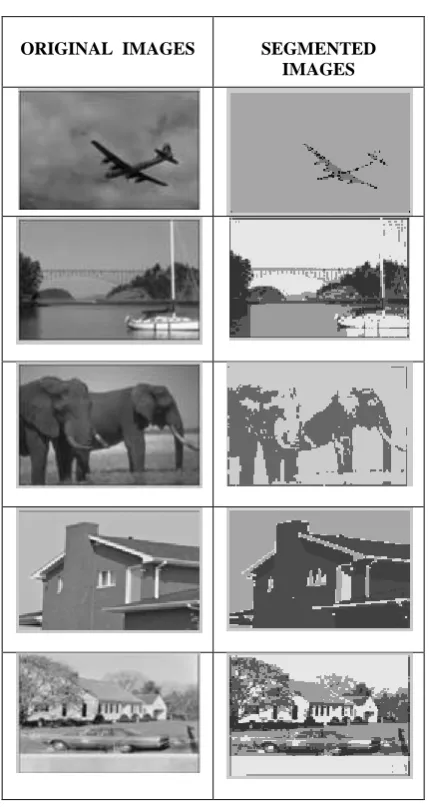
[image:8.595.60.275.267.671.2]

Using the estimated probability density function and image segmentation algorithm given in section 3, the image segmentation is done for the five images under consideration. The original and segmented images are shown in Figure 2

Fig 2: Original and Segmented Images

ORIGINAL IMAGES SEGMENTED IMAGES

7. PERFORMANCE EVALUTION

After conducting the experiment with the. By using image segmentation algorithm we have conducted the experiment and also studied its performance in this paper. The performance evaluation of the segmentation technique is

(VOI) and (iii) global consistence error (GCE). The performance of developed algorithm using Pearsonian Type I Distribution (PTID-K) is studied by computing the segmentation performance measures namely PRI, GCE, and VOI for the five images under study. The computed values of the performance measures for the developed algorithm and the earlier existing finite Gaussian mixture model(GMM) with K-means algorithm are presented in Table 4 for a comparative study.

Table 3: SEGMENTATION PERFORMACE MEASURES

IMAGES METHOD

PERFORMACE MEASURES PRI GCE VOI

FLIGHT

GMM 0.7802 0.6554 7.7477

PTID-K 0.9836 0.4702 1.9154

HOUSE

GMM 0.9028 0.7056 7.4164

PTID-K 09031 0.6963 7.3567

ELEPHANT GMM 0.9753 0.9142 8.8837

PTID-K 0.9762 0.9012 8.8270

HOUSE GMM 09252 0.6997 6.8004

PTID-K 0.9628 0.2786 6.7263

CAR GMM 0.9420 0.8779 8.8885

PTID-K 0.9559 0.8584 8.8772

From Table 3 it is identified that the PRI values of the existing algorithm based on finite Gaussian Mixture model for the five images considered for experimentation are less than that of the values from the segmentation algorithm based Pearsonian Type I distribution with K-means. Similarly GCE and VOI values of the proposed algorithm are less than that of finite Gaussian mixture model. This reveals that the proposed algorithm outperforms the existing algorithm based on the finite Gaussian mixture model.

After developing the image segmentation method and it is required to verify the utility of segmentation in model building of the image for image retrieval. The performance evaluation of the retrieved image can be done by subjective image quality testing or by objective image quality testing. The objective image quality testing methods are often used since the numerical results of an objective measure allow a consistent comparison of different algorithms. There are several image quality measures available for performance evaluation of the image segmentation method. An extensive survey of quality measures is given by Eskicioglu A.M. and Fisher P.S. (1995). For the performance evaluation of the developed segmentation algorithm, we consider the following image quality measures.

a) Average Difference = 1 1

ˆ ( , ) ( , )

M N i j

Z i j Z i j MN  

  

   

b) Maximum Distance =

Max Z i j



_

( , )



Z i j

ˆ

( , )



_

c) Image Fidelity =

2

1 1 1 1

ˆ ˆ

1 M N ( , ) ( , ) M N ( , )

i j i j

Z i j Z i j Z i j

   

   

 _  _  _ _

d) Mean Square Error = 2

1 1

1 _ˆ

( , ) ( , ) M N

j i

Z i j Z i j MN  

  

(9)

f) Image Quality Index =



2 2



2 2 ˆ 4

ˆ ( ) ( )

xy

x y

Z Z Q

Z Z

   

 

 _  _

 

where,

1 1 1 1

1 _ˆ

( , ) ;

( , )

M N M N

i j i j

Z

Z i j

Z

Z i j

MN

 

MN

 



 



 

;

2 2 2 2

1 1

1 1 _ˆ

( ( , ) ) ; ( ( , ) )

1 1

N N

x y

i i

Z i j Z Z i j Z

N N



 

     

 

1

1 _ˆ

_ˆ

( ( , )

) ( ( , )

)

1

N xy

i

Z i j

Z

Z i j

Z

N









where,

Z i j

( , )

is the pixel intensity at the pixel ( i, j ) of the original image and

Z i j

ˆ( , )

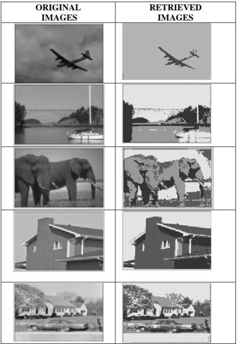
is the estimated pixel intensity at the pixel ( i, j ) of the reconstructed image .

[image:9.595.69.284.73.207.2]

Using the estimated probability density functions of the images under consideration the retrieved images are obtained and are shown in Figure 3.

Fig 3: The Original and Retrieved Images

ORIGINAL IMAGES

RETRIEVED IMAGES

The image quality measures are computed for the five retrieved images FLIGHT, BOAT, ELEPHANT, HOUSE AND CAR using the proposed model and GMM with K-means and their values are given in the Table.4

Table 4: Comparative Study of Image Quality Metrics

IMAGE Quality

Metrics

GMM

PTID-K

Standard Limits

FLIGH T

Average Difference

0.4946 0.4034 Close to 0 Maximum

Distance

1.0000 1.0000 Close to 1 Image Fidelity 1.0000 1.0000 Close to 1 Mean Square

Error

0.5011 0.4043 Close to 0 Signal to Noise

Ratio

5.6542 6.1207 As big as possible Image Quality

Index

1.0000 1.0000 Close to 1

BOAT

Average Difference

0.4946 0.0832 Close to 0

Maximum Distance

1.0000 1.0000 Close to 1

Image Fidelity 0.9000 0.9091 Close to 1 Mean Square

Error

0.4946 0.0158 Close to 0

Signal to Noise Ratio

5.6828 13.243 0

As big as possible Image Quality

Index

0.7068 0.7876 Close to 1

ELEPH ANT

Average Difference

0.4930

-43.58 59

Close to 0

Maximum Distance

1.0000 88 Close to 1

Image Fidelity 1.0000 .8395 Close to 1 Mean Square

Error

0.4930 0.4849 Close to 0

5.6897 5.7362 As big as possible Image Quality

Index

1.0011 1.0000 Close to 1

HOUSE

Average Difference

0.579 13.354 Close to 0

Maximum Distance

1.0000 1.0000 Close to 1

Error

0.5079 0.5012 Close to 0

Index

1.0007 0.9550 Close to 1

CAR

Average Difference

0.5064 13.162 2

Close to 0

Maximum Distance

1.0000 1.0000 Close to 1

Error

0.5064 0.4770 Close to 0

Index

1.0012 0.9329 Close to 1

[image:9.595.46.288.331.682.2]

(10)

the finite Gaussian mixture model by using these quality metrics.

8. CONCLUSION

This paper deals with an image segmentation algorithm based on finite mixture of Pearsonian Type I Distribution with EM + K-means algorithm. Here it is assumed that the pixel intensities of whole image follow a mixture of Pearsonian Type I Distribution. The Pearsonian Type I Distribution includes the several of the skewed distributions .The model parameters are estimated using EM algorithm , the Initialization of parameters is done through K-means and moment method of estimates. A segmentation algorithm is developed under the bayes frame. The Experiment results using Berkeley data set is revealed that this algorithm performs better then Gaussian mixture model. In image segmentation the pixel intensities of image regions are distributed asymmetrically. This is also supported by image segmentation measures such as VOI, GCE and PRI. This image segmentation method is useful in segmenting the images taken in sky and on earth.

9. REFERENCES

[1] Cheng et al (2001) “Color Image Segmentation: Advances and Prospects” Pattern Recognition, Vo1.34, pp. 2259-2281.

[2] Eskicioglu M.A. and Fisher P.S. (1995) “Image Quality Measures and their Performance”, IEEE Transactions On Communications, Vol.43, No.12, pp.2959-2965. [3] Gvs Rajkumar, K.Srinivasa Rao, And P.Srinivasa

Rao-(2011)-Image Segmentation and Retrievals based on Finite Doubly Truncated Bivariate Gaussian Mixture Model and K-Means, “Accepted for Publication” in International Journal of Computer Applications (IJCA) , Vol. 25, No. 4, pp 5-13.

[4] Jahne (1995), “ A Practical Hand Book on Image segmentation for Scientific Applications,CRC Press. [5] Kelly P.A. et al (1998), ”Statistical approach to X-ray CT

imaging and its applications in image analysis“, IEEE Trans. Med. Imag.,Vol.11, No.1, pp. 53-61.

[6] Lei T. et al (2003), “Performance Evaluation of Finite Normal Mixture Model –Based Image Segmentation Techniques”, IEEE Transactions On Image Processing, Vol-12, No.10, pp. 1153-1169.

[7] Mantas Paulinas and Andrius Usinskas (2007), “A survey of genentic algorithms applications for image enhancement and segmentation”, Information Technology and control, Vol.36, No.3, pp. 278-284. [8] M.Seshashayee, K.Srinivasa Rao, Ch.Satyanarayana And

P.Srinivasa Rao- (2011) -Image Segmentation Based on a Finite Generalized New Symmetric Mixture Model

with K – Means, International journal of Computer Science Issues,Vol.8, No.3, pp.324-331.

[9] M.Seshashayee, K.Srinivasa Rao, Ch.Satyanarayana And P.Srinivasa Rao- (2011) –Studies on Image Segmentation method Based on a New Symmetric Mixture Model with K – Means, Global journal of Computer Science and Technology, Vol.11, No.18, pp.51-58.

[10]Mclanchan G. and Peel D. (2000)), ”The EM Algorithm For Parameter Estimations ”, John Wiley and Sons, New York.

[11]Nasios N. and Bors A.G. (2006), “Variational learning for Gaussian Mixtures”, IEEE Transactions on Systems, Man and Cybernetics, Part B : Cybernetics, Vol.36(4), pp. 849-862.

[12]Pal S.K. and Pal N.R. (1993), “A Review On Image Segmentation Techniques”, Pattern Recognition, Vol.26, No.9, pp. 1277-1294.

[13]P.V.G.D.Prasad Reddy, K.Srinivasa Rao and Srinivas Yerramalle-(2007), supervised image segmentation using finite Generalized Gaussian mixture model with EM & K-Means algorithm, International Journal of Computer Science and Network Security, Vol. 7, No.4. Pp. 317-321.

[14]P.V.G.D.Prasad Reddy, K.Srinivasa Rao and Srinivas Yerramalle-(2007), supervised image segmentation using finite Generalized Gaussian mixture model with EM & K-Means algorithm, International Journal of Computer Science and Network Security, Vol. 7, No.4. Pp. 317-321.

[15]Srinivas Y. et al (2007), “Unsupervised Image Segmentation based on Finite Doubly Truncated Gaussian Mixture model with K-Means algorithm”, International Journal of Physical Sciences, Vol. 19, pp. 107-114.

[16]Shital Raut et al (2009), “Image segmentation- A State-Of-Art survey for Prediction”, International conference on Adv. Computer control, pp.420-424.

[17]SrinivasYerramalle, K.Srinivasa ao, P.V.G.D.Prasad Reddy-(2010), Unsupervised image segmentation using generalized Gaussian distribution with hierarchical clustering, Journal of advanced research in computer engineering, Vol.4, No.1 pp. 43-51.

[18]Srinivas Yerramalle And K.Srinivasa Rao-(2007), Unsupervised image classification using finite truncated Gaussian mixture model, Journal of Ultra Science for Physical Sciences, Vol.19, No.1, pp 107-114.