Social Consequences of Commitment

Munich Personal RePEc Archive

Social Consequences of Commitment

Isaac, Alan G

11 October 2006

Online at

https://mpra.ub.uni-muenchen.de/414/

Social Consequences of Commitment

An Agent-Based Approach

Author: Alan G. Isaac

Organization: Department of Economics, American University

Contact: [email protected]

Date: 2006-10-11

keywords: ACE, agent-based, computational economics, iterated prisoner’s dilemma, evolutionary prisoner’s dilemma, commitment

JEL: C63, C73

Abstract

Contents

1 Introduction 2

2 Object Oriented Programming 3

3 A Simple Game 7

4 The Prisoner’s Dilemma 10

5 CD-I Game 11

6 Evolutionary Soup 14

7 Evolutionary Grid 16

8 Commitment 18

9 Conclusion 20

10 Appendix A 20

11 References 21

1

Introduction

Computer simulation of economic interactions has been gaining adherents for more than two decades. Researchers often promote simulation methods as a “third way” of doing social science, distinct from both pure theory and from statistical exploration [axelrod1997abm]. While many methodological questions remain areas of active inquiry, especially in the realms of model robustness and of model/data confronta-tions, economists have been attracted by the ease with which computational methods can shed light on intractable theoretical puzzles. Some economists have gone so far as to argue that pure theory has little left to offer economists; that for economics to progress, we need simulations rather than theorems [hahn1991ej]. One specific hope is that simulations will advance economics by enabling the creation more realistic economic models---models that incorporate important historical and psychological proper-ties that “pure theory” has trouble accommodating, including learning, adaptation, and other interesting limits on the computational resources of economic actors. Another specific hope is that unexpected but useful (for prediction or understanding) aggregate outcomes will “emerge” from the interactions of autonomous actors. There are many examples of these hopes being met in surprising and useful ways [bonabeau2002pnas].

Economic simulations are considered to be “agent-based” when the outcomes of interest result from the repeated interaction of autonomous actors, called “agents”. These agents are autonomous in the sense that each can select actions from its own feasible set based on its own state and behavioral criteria. Agents are often stylized representations of real-world actors: either individuals, such as consumers or entrepreneurs, or aggregates of individuals, such as a corporation or a monetary authority (which may in turn be explicitly constituted of agents).

In the face of this plethora of alternatives, an additional ACE research language may seem otiose. However this paper shows that Python offers a natural environment for ACE research that should be seriously considered for ACE research and teaching. Python is a very-high-level general-purpose pro-gramming language that is well suited to ACE. This paper illustrates that suitability by quickly and simply developing a standard ACE application: the evolutionary iterated prisoner’s dilemma. The ex-ample is illustrative of the needs in ACE research, and it serves to highlight many of the advantages of Python for such research. We then show how to extend this example to explore the importance of cardinal payoffs and a possible social implication of commitment.

The iterated prisoner’s dilemma (IPD) is familiar to most social scientists, and many ACE researchers have implemented some version of the IPD as an exercise or illustration. Readers with ACE backgrounds will especially appreciate how simple, readable, and intuitive our Python implementation proves when compared to similar projects implemented in other languages. This indeed is one of the key reasons to use Python for ACE: with a little care from the programmer and an extremely modest understanding of Python by the reader, Python code is often as readable as pseudocode. This is no accident: readability is an explicit design goal of the Python language.

This paper has three related goals. First, we offer an introduction to object oriented modeling in agent-based computational economics (ACE), presenting a simple yet usable treatment of a classic ACE model. Very simple but already useful Python code is presented in the context of an evolutionary prisoner’s dilemma, illustrating our claim that ACE research finds a natural ally in the Python programming language. Second, it shows how the tools developed in this paper can be used to demonstrate the importance of cardinal payoffs in the evolutionary prisoner’s dilemma. Finally, we use the same tools to explore a possible social benefit to commitment, where ’commitment’ denotes an unwillingness to surrender a reciprocal strategy.

2

Object Oriented Programming

We will say an ’object’ is a collection of characteristics (data) and behavior (methods). We will call a computer program ’object-based’ to the extent that data and methods tend to be bundled together into useful objects. Many researchers consider models of interacting agents to be naturally object-based. For example, a player in a game is naturally conceived in terms of that individual player’s characteristics and behavior. We may therefore bundle these together into a player object. In this paper, we will consider code to be ’object-oriented’ to the extent that it relies on ’encapsulation’.1

Encapsulation means that an object’s interactions with the rest of the program is mediated by an interface that does not expose the object’s implementation details. For example, a player object may be asked for its next move by communicating with itsmovemethod, without worrying about how that method is implemented, which of its own data the player relies on to produce a move, or whether the player delegates moving to another object.

Within this highly simplified taxonomy, we can say object-oriented programming (OOP) is possible in most computer languages. It is a matter of approach and practices: OOP programming focuses on defining encapsulating objects and determining how such objects will interact. Yet it is also the case that some languages facilitate OOP. We say a programming language is object-oriented to the extent that it facilitates object-oriented programming. Key facilities of any OOP language is inheritance and polymorphism. In the roughest sense, inheritance is just one way to implement the old practice of reusing existing code: one (sub) class of objects can inherit some of its characteristics (data) and behavior (methods) from another (super) class. Inheritance proves to be an extremely powerful way to reuse existing code, and it often facilitates writing simpler and easier to understand code. Part of that simplicity arises through polymorphism, where a class determines that its subclasses respond to certain messages, but each subclasses may respond differently. For example, all player classes may implement a

movemethod, but players designed to interact on a grid may move differently than players designed for random encounters. (See the examples below.)

For ACE, the phenomenologically salient actors of economic theory will be natural objects. This adds intuitive appeal to the model: the actors in the artificial economy are autonomous units whose interactions produce the model outcomes, analogous to the real-world outcomes produced by real-world actors. This aspect of OOP may facilitate production of sensible models, and almost certainly helps with communication---two big advantages in a relatively new area of economic research. However, object

1

orientation cuts much deeper than this, and many important objects in our models will not have obvious real world counterparts. (For example, we may have objects representing player characteristics, or objects representing aggregates of economic actors, or objects storing a summary “history” of our economic model.)

Why Python?

Economists naturally care about how the choice of a programming environment affects productivity: how quickly and painlessly can we implement a given idea in a given environment? The choice of programming language will often be very personal, responding to individual modes of thinking and to existing human capital. However many ACE researchers have claimed that OOP languages facilitate ACE modeling. And as we will see, one of the great appeals of Python is its ease of use and natural syntax, which allows rapid learning and easy prototyping. Among object-oriented languages, Python has some specific advantages for agent-based modeling. No one advantage makes Python unique, but together they add up to an attractive combination of power and ease of use.

Interpreted Language It is widely acknowledged that interpreted languages can facilitate prototyping and rapid development. They can also facilitate learning (due to the immediate feedback from the interpreter). Python interpreters exist for every major platform. This means that Python code is largely platform independent, which in turn facilitates code-sharing and collaboration with other ACE researchers.

Dynamic Typing Like many interpreted languages, Python is dynamically typed: variables (names) do not have types; rather the values that are assigned to them do. Here we emphasize two positive aspects of dynamic typing: code becomes simpler to write and simpler to read, and prototyping and refactoring are facilitated. (Many statically typed languages lack type inference, which leads to programs that appear cluttered with type declarations and explicit casts.)

Duck Typing Python encourages programming to objects’ methods rather than to their types. This in turn encourages a strong polymorphism known as duck typing: functions and classes interact objects based on their attributes (rather than their class). Again, rather than engaging the varied controversies over duck typing, we simply note a widely acknowledged advantage: it facilitates quick prototyping and refactoring.

Garbage Collection Many languages require the programmer to explicitly allocate and deallocate memory for any objects created. Memory leaks are a common problem in such languages, even for experienced programmers. Other languages, Python included, offer automatic memory manage-ment: garbage collection ensure that memory is freed up when the object stored there is no longer needed. This can involve some sacrifice of speed and memory usage, but the gain in convenience is considerable.

Powerful Standard Library Python comes with a powerful, and extremely well documented standard library. Two component of special interest to ACE researchers will be the utilities for platform independent interaction with the operating system and the extensive random-number services. (Random number generation uses the Mersenne Twister by default.)2

Flexible Data Structures Python provides a collection of powerful and flexible data structures. Here we mention sequence data types and dictionaries.3

Note that, as a result of Python’s strong object orientation, these types are easily subclassed and extended when needed.

Sequence data types are indexed collections of items, which may be heterogeneous. Lists and tuples are sequence types that are ubiquitous in Python programming. Lists are very flexible: they can grow or shrink, and can hold heterogeneous elements. An empty list can be created as []or as

list(). Elements can then be added with the append method. A populated list can also be created directly by listing its elements between brackets, for example[1,’a’]is a two element list (with heterogeneous elements). A list of lists can be a natural representation of a two-dimensional array, such as a grid or a matrix.4

Sequences can be used for loop control: Python’s for statement iterates over the items of a se-quence. For example, if x is a list or tuple, the following code snippet prints a representation of each item inx:

2

f o r item i n x : p r i n t item

Like many programming languages, Python uses zero-based indexing: if x is a sequence, then

x[0] returns the first element of x.5

To illustrate zero-based indexing in more detail, consider the statement payoffmat = [ [(3,3),(0,5)] , [(5,0),(1,1)] ](which occurs in our code exam-ples below). This is a list of two lists of two tuexam-ples each. Since we index sequence elements by postfixing an integer in brackets,payoffmat[0]is[(3,3),(0,5)]. Similarly,payoffmat[0][1]is

(0,5). (This tuple represents two player payoffs given moves 0 and 1.)

Lists are “mutable”: you can replace list items by assignment. For example, if x is a list, then

x[0]=99 will set the first element of x to the integer 99. Tuples are “immutable”: you cannot replace list items by assignment. For example, if xis a tuple, thenx[0]=99will raise an error. The dictionary is the basic Python mapping data type (resembling hash tables or associative arrays in other languages). A dictionary is a collection of key-value pairs, where the value can be retrieved by using the key as an index. If x=dict(a=0,b=1) then x[’a’] returns the value 0. The same dictionary can be created from a list of 2-tuples: x=dict( [(’a’,0), (’b’,1)] ), which will often prove useful.

Useful “Built-In” Functions A few dozen very useful functions are built-in to Python, in the sense that they are always available. The user does not need to import any standard library modules to access these functions. We will mention three at this point: range,enumerate, and zip.

If nis a nonnegative integer, then range(n)creates a list of the firstnnonnegative integers. It is idiomatic in Python to userangefor loop control: e.g.,for i in range(10): print i. Ifxis a sequence, thenenumerate(x)pairs each element with its index. For example, ifx=[9,8,7]

thenenumerate(x)will generate the tuples (0,9), (1,8), and (2,7). (Recall from above that Python uses zero-based indexing.)

If xis a sequence andyis a sequence, then zip(x,y)will produce a list of 2-tuples, pairing each element ofxwith the corresponding element of y. For example, If x=(9,8,7)andy=(6,5,4)then

zip(x,y)creates the list[(9,6), (8,5), (7,4)].

Let us call that last list z. If we now evaluate zip(*z) we create the list [(9,8,7),(6,5,4)], which contains our two original tuples. The asterisk instructs Python to “unpack”zso as to use each element of zas an argument of zip. Note that this means thatzipcan be used to transpose a list of equal length lists.

We will often usezipto construct dictionaries in a particularly compact yet readable way. Suppose

playersis a list of players andmovesis a corresponding list of moves. Thenzip(players,moves)

produces a list of 2-tuples by “zipping” together each player and its move. A dictionary can be initialized with such a list of 2-tuples. So d=dict( zip(players,moves) ) produces a mapping from players to moves. We will use this compact and readable idiom repeatedly.6

Generator Expressions Python has evolved some very powerful and easy to read syntax for the cre-ation of data structures. Rather than traditional looping constructs, “generator expressions” are often preferred for producing lists and tuples. Generator expressions are perhaps best introduced by example.

Suppose players is a tuple of players, each of whom has a playertype attribute, and we want to produce a corresponding tuple of playertypes. Here is a (fairly) traditional approach to this problem:

3

For a detailed and generally excellent introduction, see the Python Tutorial.

4

However, efficient computations with multi-dimensional arrays will generally use the numpy package.

5

Zero-based indexing can initially feel odd to those with no programming experience (even though we use it all the time when referring, e.g., to the 21st century). In practice, it proves extremely convenient.

6

p t y p e s = l i s t ( )

f o r p l a y e r i n p l a y e r s :

p t y p e s . append ( p l a y e r . p l a y e r t y p e ) p t y p e s = t u p l e ( p t y p e s )

Here we create an empty list, to which we sequentially append the playertype type of each player, and we finally create a tuple corresponding to the list of playertypes. (Note the attribute accesses, which use the “dot notation” common in object oriented languages.) We can accomplish the same thing more elegantly and efficiently with a generator expression:

p t y p e s = t u p l e ( p l a y e r . p l a y e r t y p e f o r p l a y e r i n p l a y e r s )

This iterates through the generator(player.playertype for player in playerlist)to popu-late a tuple of player types, one playertype for each player.7

The expression on the right reads very naturally: create a tuple that contains the player’s playertype for each player in players. This is a beautifully readable and compact way to generate this tuple’s elements.

Graphics Excellent and powerful graphics libraries are available. For example, users needing interactive two-dimensional graphs might use the Matplotlib package, which allows both ease of use and, for those who need it, a remarkably fine-grained control of graphical presentations.

Numerics The numpy package implements powerful multidimensional arrays along with the basic func-tionality required for scientific computing. The numpy-based SciPy package offers substantial additional functionality, resulting in a free and open source scientific computing environment com-petitive with many commercial offerings.

Extensibility As with other interpreted languages, speed concerns arise when Python programs make heavy use of looping constructs. The high speed of modern computers moderate this concern but for models with very large numbers of agents does not eliminate it. Fortunately it is easy to write Python performance enhancing extensions in relatively low-level programming languages such as C or Fortran.8

String Formatting Python string interpolation can be done in standard C language (printf) fashion, but interpolation values can also be provided as a dictionary (i.e., a hash table). This makes for convenient report generation (e.g., when objects are asked about their current state).

Documentation Online documentation is excellent and free. In addition Python encourages the cre-ation of self-documenting objects, and most built-in functions provide excellent self-documentcre-ation.

Readability For write-once read-never code, readability is perhaps not an issue. For code that is to be shared with a research community and reread after the passage of time, readability is a crucial consideration. Python code is often as readable as pseudocode, as we shall see. Readability is aided by Python’s syntax, especially the use of whitespace to delimit code blocks.9

It is also aided by the Python “culture”, which emphasizes code readability and disparages clever programming “tricks”.

Free and Open Source It is easy to exaggerate the importance of the financial cost of software, which is usually a small relative the the cost of doing research. More important is the freedom to modify: the licenses of most Python packages allow users to change them as needed. This is even true of the excellent graphics and numerical packages. The open source nature of the software makes this freedom relevant: users often contribute enhancements to important packages. Finally, some re-searchers plausibly claim that the use of closed source software conflicts with the goal of verifiability and replicability in science.

7

An attentive reader might wonder why the generator example has only a single pair of parentheses. When a generator expression when it is the only argument of a function, Python allows us to omit its parentheses.

8

See for example the ctypes module, f2py, Pyrex, SWIG, and weave.

9

Other important features of Python---exception handling, support for unit testing, support for multi-ple inheritance, support for metaclasses, support for metaprogramming (via descriptors such as decorators and properties), support for sophisticated operator overloading, and memory conserving features such as slots---may prove useful in advanced applications. Some limitations of Python are relevant for projects with very large numbers of agents---as an interpreted language Python will lack the speed of many com-piled languages, and Python’s restrictions on running process-bound threads on multiple processors may prove a restriction (on a single machine) in very special circumstances.10

These issues are beyond the scope of the current paper.

3

A Simple Game

When discussing computational economics, nothing substitutes for actual code, so we will now create a very simple game. We do not address game theoretic considerations at this point: our two players will randomly chose their moves and ultimately receive the payoffs determined by the game.

For this first very simple game, we introduce only two types of object: a game, and players. Each object will instantiate a class, which encapsulates its characteristics (accessible via data attributes) and behavior (elicited via method attributes).11

To allow a simple introduction to Python classes, we will strive for almost trivial classes in our first simple game. For example, our first players will be instances of aRandomMoverclass. When asked for a move, aRandomMoverinstance will do little more than generate a random value and test it against a probability of defection.

# L i s t i n g : simple game . py

from u s e r u t i l s import ∗ #u t i l i t i e s : mean , t r a n s p o s e , and random

c l a s s RandomMover :

p = 0 . 5 #p r o b a b i l i t y o f d e f e c t i o n d e f move ( s e l f , game ) :

r e t u r n random ( ) < s e l f . p d e f r e c o r d ( s e l f , game ) :

p a s s

c l a s s SimpleGame :

payoffmat = [ [ ( 3 , 3 ) , ( 0 , 5 ) ] , [ ( 5 , 0 ) , ( 1 , 1 ) ] ] d e f i n i t ( s e l f , p l a y e r 1 , p l a y e r 2 ) :

s e l f . p l a y e r s = [ p l a y e r 1 , p l a y e r 2 ]

s e l f . opponents = {p l a y e r 1 : p l a y e r 2 , p l a y e r 2 : p l a y e r 1}

d e f run ( s e l f , m a x i t e r =4):

#c r e a t e an empty l i s t t o s t o r e t h e h i s t o r y o f moves s e l f . h i s t o r y = l i s t ( )

f o r c t i n r a n g e ( m a x i t e r ) :

#g e t t h e new move f o r each p l a y e r

newmove = t u p l e ( p l a y e r . move ( s e l f ) f o r p l a y e r i n s e l f . p l a y e r s ) #append t h e new p l a y e r moves t o t h e h i s t o r y l i s t

s e l f . h i s t o r y . append ( newmove ) f o r p l a y e r i n s e l f . p l a y e r s :

#each p l a y e r can r e c o r d game i n f o ( e . g . , t h i s game p l a y e d ) p l a y e r . r e c o r d ( s e l f )

d e f p a y o f f ( s e l f ) :

#make t u p l e : a p a y o f f−p a i r f o r each move−p a i r

m o v e p a y o f f s = t u p l e ( s e l f . payoffmat [ m1 ] [ m2 ] f o r (m1, m2) i n s e l f . h i s t o r y ) #t r a n s p o s e move p a y o f f s t o g e t l i s t o f p l a y e r p a y o f f s

p l a y e r p a y o f f s = t r a n s p o s e ( m o v e p a y o f f s ) #compute mean p a y o f f f o r each p l a y e r

10

See http://blog.ianbicking.org/gil-of-doom.html for an accessible discussion.

11

a v e r a g e p a y o f f = t u p l e ( mean ( p a y o f f ) f o r p a y o f f i n p l a y e r p a y o f f s ) #p a i r each p l a y e r with i t s p a y o f f

p l a y e r s w i t h p a y o f f s = z i p ( s e l f . p l a y e r s , a v e r a g e p a y o f f ) #r e t u r n a mapping : p l a y e r −> p a y o f f

r e t u r n d i c t ( p l a y e r s w i t h p a y o f f s )

The listing labeled simple_game.pycontains the defintion of the RandomMover class. (Readers fa-miliar with class and function definitions can skim the next few paragraphs.) A class definition starts with the keywordclass, followed by the name (RandomMover) that we are giving the class, followed by a colon.12

So the line class RandomMover: begins our definition of the RandomMover class, which is completed by the indented statements that follow. The first statement,p = 0.5, creates a data attribute that will be shared by all instances of the class. The variablep will be the probability of choosing the “defect” strategy. Since this data is shared by all instances, we call it a “class attribute”. (For more

detail, see the Python tutorial.)

The next statement is a function definition. Recall that blocks are defined in Python by level of indentation (and never, e.g., by the use of braces), so these function definitions must be indented to make them part of the class definition. (Similarly, the body of each function definition is given an

additional _{level of indentation.)}

A function definition starts with the keyword def, followed by the name that we are giving the function, followed by a (possibly empty) list of function parameters in parentheses, followed by a colon. Naturally, the function parameters are names that arelocal _{to the function definition. (So they will not}

conflict with the same names used elsewhere in our program.)

So the line def move(self,game): begins our definition of the move function. Clearly we named the function movebecause it generates the player moves. The function has two arguments. The second argument, namedgame, will be ignored byRandomMoverinstances but used by other player types (below). The first argument is calledself, for reasons that we now discuss.

Recall that the function parameter self is a name that is local _{to the function definition. We can}

therefore freely choose a name for this argument of our function, but when the function definition is part of a class definition, it is conventional name the first argument self. This is because functions defined in our class become the methods of instances of the class, and a method always receives as an implicit first argument the instance on which it is called. (This is likely to sound obscure to a reader with no OOP background, but it should be clear by the end of this section.)

Next comes the body of the function, which in this case is a single statement: return random() < self.p. When this return-statement is executed, the function returns the boolean (True or False) value

random() < self.p. This value it is computed as follows. The expressionrandom()evaluates to a draw from a standard uniform distribution, so it is a floating point number between zero and one.13

The expressionself.pwill retrieve the pattribute of self. The inequality comparison value is either True or False. We interpret True as “defect” and False as “cooperate”.

The other class in simple_game.pyisSimpleGame. ASimpleGameinstance has more data and more methods, and it uses some new data structures, so we will approach it more slowly.

As usual, we begin our class definition with the statement class SimpleGame:. We then create a payoff matrix as a class attribute: payoffmat = [ [(3,3),(0,5)] , [(5,0),(1,1)] ]. This payoff matrix is created using two useful Python array-like data types: lists and tuples. (See the discussion of data types above.) The payoff matrix is a list of two lists, where each inner list contains two tuples. These tuples hold the move-based payoffs for two players. For example, the tuple(3,3)gives the payoffs to the players if both cooperate: for that move, each player gets a payoff of 3. In subsequent sections, we will consider the payoff matrix in much more detail.

Next we do something new: we introduce a function to initialize instances of the SimpleGame class. The name__init__is special: it is the name that must be used for the function that does the “initial-ization” when a new instance is created. We will call this the ’initialization function’ for the class. In the initialization function, we have an opportunity to set initial values for instance attributes: in this case, a data attribute of the particular instance. We initialize anySimpleGameinstance with two player instances. These will be the players for that game.

The __init__ function of SimpleGame has three parameters: self, player1, and player2. As discussed above,selfwill be the local name of the instance that is being initialized. Similarly, the player

12

In this paper we consider only classic classes.

13

The functionrandomcan be found in therandommodule of the Python standard library. (At the top ofsimple_game.py

instances we pass in will have the local namesplayer1andplayer2. So the statementself.players = [player1,player2]creates an attribute named playersfor the instanceselfand assigns as its value a list of the players we pass to the __init__ function. Similarly, the statement self.opponents = {player1:player2, player2:player1} creates a mapping (from each player to the other, i.e., to the “opponent”) and assigns it to the opponents attribute of the game (self.opponents). (This mapping

will prove useful in later sections.)

Once we have an initialized SimpleGame instance, we can do two things with it. We can run the game by calling the instance’s runmethod, and after that we can get the game payoff for each player by calling the payoff method. The associated code is very heavily commented and therefore largely self explanatory. Note that each time we run a game, the game records the history of the moves made. Naturally, this history of moves determines the game’s payoff.

Recalling our earlier discussion of generator expressions, we see that the definition of run includes the a generator expression in tuple( player.move() for player in self.players ). Our earlier discussion explained that this expression will create a tuple as follows: for each player in in the game (i.e., inself.players), create a tuple element that is that player’s move.

Now that we have written our two classes, we want to use them to run a game. A file containing Python code that can be imported is called a module. We canimportobjects from a module into any program we wish. Consider the following code, which will run our first game. Note that it begins by importing everything (*) from the simple_game module, thus making available the RandomMover and

SimpleGameclasses.

# L i s t i n g : p l a y s i m p l e g a m e . py

from simple game import ∗

#c r e a t e two p l a y e r s p l a y e r 1 = RandomMover ( ) p l a y e r 2 = RandomMover ( ) #c r e a t e and run t h e game

game = SimpleGame ( p l a y e r 1 , p l a y e r 2 ) game . run ( )

#r e t r i e v e and p r i n t t h e p a y o f f s p a y o f f s = game . p a y o f f ( )

p r i n t p a y o f f s [ p l a y e r 1 ] , p a y o f f s [ p l a y e r 2 ]

Our program for running the game is very simple. We start by creating two “players”---that is,

RandomMover instances. A class in Python is a callable object; it returns an instance of the class when called. In order to produce aRandomMoverinstance, we call theRandomMoverclass by appending parentheses (just as when calling a function). So the expressionRandomMover()creates a RandomMover

instance. The two players in our game are “instances” of the RandomMover class. (We say that each player “instantiates” theRandomMoverclass.)

Once we have our two players (namedplayer1andplayer2), we can create aSimpleGamefor them to play: game = SimpleGame([player1,player2]). Note that this we call the class SimpleGame with two arguments: the two player instances required by the initialization function. When a SimpleGame

instance is created, its __init__method is called with these arguments to initialize the instance. We defined this initialization to do one thing: it sets the value of theplayersattribute of ourSimpleGame

instance to a list containing our players. Note that it is the instance, not the class, which owns this data. Finally we are ready to run our game and print the resulting payoffs. Therunmethod of an instance of SimpleGameruns the game (when called). The game requests moves from the players, records their moves as the game history, and determines the game payoffs as the average of the move payoffs.

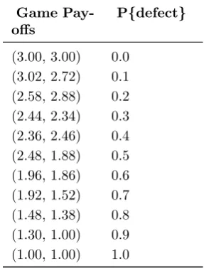
Table 1: Game Payoffs at Various Defection Probabilities

Game Pay-offs

P{defect}

(3.00, 3.00) 0.0 (3.02, 2.72) 0.1 (2.58, 2.88) 0.2 (2.44, 2.34) 0.3 (2.36, 2.46) 0.4 (2.48, 1.88) 0.5 (1.96, 1.86) 0.6 (1.92, 1.52) 0.7 (1.48, 1.38) 0.8 (1.30, 1.00) 0.9 (1.00, 1.00) 1.0

After analyzing just a few lines of code, many readers may find that Python programs are already becoming easy to read, so even nonprogrammers may now be feeling ready to try their hand at writing some code. This readability and simplicity is quite an astonishing strength of Python. What is more, our barebonesSimpleGameclass has enough features that it will remain useful throughout this paper.

4

The Prisoner’s Dilemma

Our next project is to explore the consequencies of strategy choice in an iterated prisoner’s dilemma. In a simple prisoner’s dilemma there are two players each of whom has two strategies, traditionally called ’cooperate’ (C) and ’defect’ (D). The payoffs are such that---regardless of how the other player behaves---a player always achieves a higher individual payoff by defecting. However the payoffs are also such that when both players defect they each get an individual payoff less than if both had cooperated.

Real world applications of the prisoner’s dilemma are legion [poundstone1992]. One unusual illus-tration considers a practice of competitive wrestlers: food deprivation and even radical restriction of liquids in an effort to lose weight in the days before a weigh-in. This is followed by rehydrating and binge eating after the weigh-in but before the match. Whether or not other wrestlers also follow this regime, individual wrestlers perceive it to provide a competitive advantage. But it is plausible that all players would be better off if the practice were ended (perhaps by requiring a weigh-in immediately before the match).

In its game theoretic formulation, stripped of the social ramifications of betrayal, the prisoner’s dilemma suffers from a misnomer: there is a dominant strategy so there is no dilemma, and each player chooses without difficulty the individually rational strategy. Economists may be inclined to call this game “the prisoners paradox”, to highlight the failure of individually rational action to produce an efficient

outcome. In the present paper we nevertheless stick with the conventional name.

The payoff matrix in our SimpleGame is a very common representation of the prisoner’s dilemma, common enough to be called canonical. We can use these payoffs to highlight the paradoxical nature of the prisoner’s dilemma. Imagine that the game is played in three “countries” filled with different kinds of players. The population of the Country A comprises random players, as in ourSimpleGameabove, that choose either of the two strategies with equal probability. The average payoff to individuals in Country A is 2.25. People in Country B are instrumentally rational individuals: they act individually so as to produce the best individual outcome, without knowledge of the other player’s strategy. (That is, each player always chooses to defect.) The average payoff to individuals in Country B is 1. People in Country C have somehow been socialized to cooperate: each individual always chooses the cooperative strategy. The average payoff to individuals in Country C is 3.

Defining the Prisoner’s Dilemma

Some authors define the prisoner’s dilemma to include two additional constraints on the payoff matrix: the matrix must be symmetric, and the payoff sum when both cooperate must be at least the payoff sum when one cooperates and the other defects. [rapoport chammah-1965] introduce the latter restriction, which is sometimes justified as capping the payoff to defection or reducing the attractiveness of a purely random strategy. Many authors simply use without discussion the traditional payoff matrix above, which satisfies these constraints. As we shall see, even within these constraints, payoffs matter.

5

CD-I Game

When game payoffs resemble a prisoner’s dilemma, observations of cooperative behavior are provocative: they may indicate deviations from the individually rational equilibrium, or they may indicate that the payoffs have been incorrectly understood [rapoport chammah-1965]. In 1971, [trivers-1971-qrbio] pro-posed reciprocity as a basis of cooperation. A decade later, political science and evolutionary biology joined hands to show that reciprocity could serve a basis for cooperation even in the face of a prisoner’s dilemma [axelrod hamilton-1981science]. This led to the exploration of the iterated prisoner’s dilemma, wherein players play a prisoner’s dilemma repeatedly. Unlike the static version, an iterated prisoner’s dilemma can actually involve a dilemma: defecting will raise the one period payoff but may lower the ultimate payoff. (An evolutionary aspect arises when strategy success influences strategy persistence; we will address this in subsequent sections.)

We now consider slightly more complex player types, using a characterization that is common in the literature. A playertype is characterized by a rule for initial action and by rules for reacting to past events: the likelihood of defection depends on whether the player faced cooperation of defection on the previous move of the game. Such players care whether the other player cooperated (C), the other player defected (D), or players are making their initial move (I). We will therefore call this the CD-I playertype. The CD-I playertype will be parameterized by a 3-tuple of probabilities: the probability of defecting when the other cooperated on the previous move, the probability of defecting when the other defected, and the probability of defecting on the initial move. The game played will again be iterations of our prisoner’s dilemma.

An implementation of this is found in thesimple_cdi.pylisting. Once again the basic idea will be to create a game with two players. We will use this opportunity to illustrate delegation and inheritance. Note that we replace theRandomMoverclass with two classes: theSimplePlayerclass and theSimpleCDIType

class. That is, we separate out the notion of a “player” and a “playertype”.

# L i s t i n g : s i m p l e c d i . py

from simple game import ∗

c l a s s S i m p l e P l a y e r :

d e f i n i t ( s e l f , p l a y e r t y p e ) : s e l f . p l a y e r t y p e = p l a y e r t y p e s e l f . r e s e t ( )

d e f r e s e t ( s e l f ) :

s e l f . games played = l i s t ( ) #empty l i s t s e l f . p l a y e r s p l a y e d = s e t ( ) #empty s e t d e f move ( s e l f , game ) :

#d e l e g a t e move t o p l a y e r t y p e

r e t u r n s e l f . p l a y e r t y p e . move ( s e l f , game ) d e f r e c o r d ( s e l f , game ) :

s e l f . games played . append ( game )

s e l f . p l a y e r s p l a y e d . add ( game . opponents [ s e l f ] )

c l a s s SimpleCDIType : p = ( 0 . 5 , 0 . 5 , 0 . 5 )

d e f move ( s e l f , p l a y e r , game ) : o t h e r = game . opponents [ p l a y e r ]

i f other move i s None :

newmove = ( random ( ) < s e l f . p [−1 ] ) e l s e :

newmove = ( random ( ) < s e l f . p [ other move ] ) r e t u r n newmove

c l a s s CDIGame( SimpleGame ) :

d e f f e t c h m o v e ( s e l f , p l a y e r , t ) : i f s e l f . h i s t o r y :

p l a y e r i d x = s e l f . p l a y e r s . i n d e x ( p l a y e r ) move = s e l f . h i s t o r y [ t ] [ p l a y e r i d x ] e l s e :

move = None r e t u r n move

Let us first examine theSimplePlayerclass. ASimplePlayerinstance must have a playertype, as can be seen by the__init__function: initialization involves setting theplayertype attribute for the Sim-plePlayer instance. (The line self.playertype = playertypeassigns the value of the local variable namedplayertypeto the instance attribute of the same name, which is accessed as self.playertype.) During initialization, we also call reset to create a games_played attribute and a players_played

attribute. (Since games know their players, theplayers_playedattribute is in a sense redundant, but it will prove convenient.) These will serve as player “memory”, which will be added to when the players

recordmethod is invoked by a game. (Recall that therunmethod of aSimpleGameinstance will invoke the recordmethod for each player.) Looking at the move function, we see that a player delegates its moves to its playertype: this is our first use of delegation, a common strategy in object oriented pro-gramming. (Note that when a player calls themovemethod of its playertype instance, it passes itself to the playertype. This means that, when determining a move, the playertype has access to player specific information.)

Next consider ourSimpleCDITypeclass, which constructs our player type instances. The SimpleCDI-Typeclass has a class attribute,p, just as theRandomMoverclass did. Indeed, since we set all the elements of p to 0.5 in this class attribute, the basicSimpleCDIType determines moves in the same way as our

RandomMoverdid. This can be seen by working through the movefunction for this class. For the initial move, the probability of defection is given by the last element of the tuplep(which we can index with -1). After the initial move, the probability of defection is conditional on the last move of the other player. (Note that the playertype fetches this move from the history of the player’s game; see theCDIGamecode for the details.) If the other player cooperated, the first element of pis the probability of defection. If the other player defected, the second element of pis the probability of defection.

Finally we consider ourCDIGameclass, which constructs our game instances. Notice that theCDIGame

class is only partly specified. When we begin our class definition asclass CDIGame(SimpleGame): we “inherit” data and behavior from theSimpleGame class. Specifically, we inherit the __init__, runand

payofffunctions, as well as the payoffmat class attribute. The use of inheritance is the typical idiom for code reuse in object oriented programming: we reuse data and behavior specified in theSimpleGame

class definition.

Recall from the__init__function in theSimpleGameclass definition that a game is initialized with two players. When run, the game is recorded by eachSimplePlayerinstance in its games_playedlist. This is what allows a player type to determine the player’s move: when a player delegates a move to its player type, the playertype fetches from the game theother _{player’s last move (i.e., the move with}

index -1). This is accomplished by invoking the game’sfetch_movemethod. (Recall that the probability of defection generally is conditional on the other player’s last move.) The fetch_move function in the

CDIGame class definition provides the needed move fetching functionality by returning the appropriate element of the game’s move history.

history, these linkages appear natural.14

With our new class definitions in hand, we are ready to create playertypes, players, and a game. Of course we can construct an endless variety of CD-I playertypes. The present paper considers only the pure strategies: each element of the strategy 3-tuple is either zero or one. This gives us 8 possible player types and therefore 36 different games. (There are 36 unique pairings, since player order is irrelevant.) The listingplay_simple_cdi.pyconducts a round robin tournament, in the sense that it produces the outcomes for all these possible pairings. We will work through the code and then suggest a conclusion.

# L i s t i n g : p l a y s i m p l e c d i . py

from s i m p l e c d i import ∗

C,D = 0 , 1 #always c o o p e r a t e ( 0 ) o r always d e f e c t ( 1 ) PURE STRATEGIES = [ (C, C,C) , (D, C,C) , (C, D,C) , (D, D, C) ,

(C, C,D) , (D, C,D) , (C, D,D) , (D, D,D) ]

#c r e a t e two p l a y e r type i n s t a n c e s

ptype1 , ptype2 = SimpleCDIType ( ) , SimpleCDIType ( ) #c r e a t e two p l a y e r s , one f o r each p l a y e r type

p l a y e r 1 , p l a y e r 2 = S i m p l e P l a y e r ( ptype1 ) , S i m p l e P l a y e r ( ptype2 ) #c r e a t e a game f o r t h e two p l a y e r s t o p l a y

game = CDIGame( p l a y e r 1 , p l a y e r 2 )

#p l a y a game f o r each p a i r o f s t r a t e g i e s

f o r i , s t r a t e g y 1 i n enumerate (PURE STRATEGIES ) : f o r j i n r a n g e ( i +1):

s t r a t e g y 2 = PURE STRATEGIES [ j ] #a s s i g n s t r a t e g i e s t o p l a y e r t y p e s

ptype1 . p , ptype2 . p = s t r a t e g y 1 , s t r a t e g y 2 p r i n t ”\nRun Game”

game . run ( )

p a y o f f s = game . p a y o f f ( )

p r i n t s t r a t e g y 1 , p a y o f f s [ p l a y e r 1 ] p r i n t s t r a t e g y 2 , p a y o f f s [ p l a y e r 2 ]

As a preliminary, we create a list of all eight pure strategies in the CDI game. We create two

SimpleCDITypeplayer type instances, and then two players (initialized with our two player types), and finally we create a game for our two players to play. We then play the game for each pair of strategies and print the results of these games.15

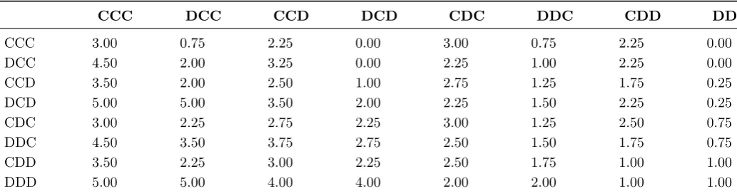
Table 2 summarizes the payoffs to the first player in each of these 36 games.

Table 2: Player 1 Payoffs with Different Strategies

CCC DCC CCD DCD CDC DDC CDD DDD

CCC 3.00 0.75 2.25 0.00 3.00 0.75 2.25 0.00

DCC 4.50 2.00 3.25 0.00 2.25 1.00 2.25 0.00

CCD 3.50 2.00 2.50 1.00 2.75 1.25 1.75 0.25

DCD 5.00 5.00 3.50 2.00 2.25 1.50 2.25 0.25

CDC 3.00 2.25 2.75 2.25 3.00 1.25 2.50 0.75

DDC 4.50 3.50 3.75 2.75 2.50 1.50 1.75 0.75

CDD 3.50 2.25 3.00 2.25 2.50 1.75 1.00 1.00

DDD 5.00 5.00 4.00 4.00 2.00 2.00 1.00 1.00

Perhaps the most striking thing about Table 2 is that playing DD-D produces a maximal payoff in all

14

We can also endow players with memories, which can deviate unreliably from the game history or be limited in capacity. We do not explore these possibilities in the present paper.

15

but two cases: when pitted against the strategies CD-C and CD-D. Put in simple terms, DD-D would be dominant if the imitative/reciprocal strategies where removed from the strategy space. (These strategies are imitative in that they always adopt the opponent’s previous move. They are reciprocal in that they always respond in kind.) The first of these, CD-C, is the famous Tit-For-Tat strategy. The robustness of this strategy in an IPD context has been long recognized [axelrod hamilton-1981science]. Neither of these two strategies dominates the other. It is however noteworthy that CD-D holds its own against DD-D, whereas CD-C does not. Note too that two CD-C players will do much better than two CD-D players.16

The subsequent sections explore some consequences of these observations.

6

Evolutionary Soup

We now consider a simple evolutionary mechanism: players are inclined to adopt winning strategies. Our first implementation of these evolutionary considerations will be in the context of random encounters between players. We introduce simple representations of a round and a tournament. A tournament consists of several rounds. On each round, players are randomly sorted into pairs, and each pair plays a CDIGame. After playing a game, a player switches (with some probability) to a winning strategy (for that game). We will characterize how an initially diverse group of players evolves over time.

The filesimple_soup.pycontains new classes to implement this evolutionary tournament. There are three classes: SoupPlayer,SimpleRound, andSimpleTournament. (The game played will be unchanged:

CDIGame.)

# L i s t i n g : s i m p l e s o u p . py

from s i m p l e c d i import ∗

c l a s s SoupPlayer ( S i m p l e P l a y e r ) : s e l e c t i o n p r e s s u r e = 1 d e f c h o o s e n e x t t y p e ( s e l f ) :

p l a y e r s = s e t ( s e l f . p l a y e r s p l a y e d ) p l a y e r s . add ( s e l f )

b e s t t y p e s = f i n d b e s t p l a y e r t y p e s ( p l a y e r s ) s e l f . n e x t p l a y e r t y p e = randomchoice ( b e s t t y p e s ) d e f e v o l v e ( s e l f ) :

i f random ( ) < s e l f . s e l e c t i o n p r e s s u r e : s e l f . p l a y e r t y p e = s e l f . n e x t p l a y e r t y p e

d e f g e t p a y o f f ( s e l f ) : #c a l l e d by f i n d b e s t p l a y e r t y p e s ( ) p a y o f f = 0

f o r game i n s e l f . games played : p a y o f f += game . p a y o f f ( ) [ s e l f ] r e t u r n p a y o f f

c l a s s SimpleRound :

d e f i n i t ( s e l f , p l a y e r l i s t ) : s e l f . p l a y e r s = p l a y e r l i s t d e f run ( s e l f ) :

s e l f . p r e p a r e p l a y e r s ( ) s h u f f l e ( s e l f . p l a y e r s )

f o r g a m e p l a y e r s i n g r o u p s o f ( s e l f . p l a y e r s , 2 ) : game = CDIGame( ∗g a m e p l a y e r s )

game . run ( )

s e l f . e v o l v e p l a y e r s ( ) d e f p r e p a r e p l a y e r s ( s e l f ) :

f o r p l a y e r i n s e l f . p l a y e r s : p l a y e r . r e s e t ( )

d e f e v o l v e p l a y e r s ( s e l f ) :

f o r p l a y e r i n s e l f . p l a y e r s :

16

p l a y e r . c h o o s e n e x t t y p e ( ) f o r p l a y e r i n s e l f . p l a y e r s :

p l a y e r . e v o l v e ( )

c l a s s SimpleTournament : nrounds = 10

Round = SimpleRound

d e f i n i t ( s e l f , p l a y e r l i s t ) : s e l f . p l a y e r s = p l a y e r l i s t d e f run ( s e l f ) :

p l a y e r s = s e l f . p l a y e r s

s e l f . p l a y e r t y p e h i s t o r y = l i s t ( ) #empty l i s t s e l f . r e c o r d ( ) #r e c o r d p l a y e r t y p e c o u n t s round = s e l f . Round ( p l a y e r s )

f o r i i n r a n g e ( s e l f . nrounds ) : round . run ( )

s e l f . r e c o r d ( ) #r e c o r d p l a y e r t y p e c o u n t s d e f r e c o r d ( s e l f ) :

c o u n t s = c o u n t p l a y e r t y p e s ( s e l f . p l a y e r s ) s e l f . p l a y e r t y p e h i s t o r y . append ( c o u n t s )

The SoupPlayer class inherits much of its behavior fromSimplePlayer, but it has new attributes deriving from our desire that it be able to evolve its playertype. When we call the choose_next_type

method of aSoupPlayer instance, this sets thenext_player_typeattribute. (The next_player_type

is always set to a winning playertype, as determined by a find_best_playertypes utility, which calls the get_payoff method of each player.) However a player instance does not change its playertype until itsevolvemethod is called. At that point, the theselection_pressureattribute determines the probability of adopting thenext_player_type. (We letselection_pressure be a class variable with value 1; with this default the player will always adopt itsnext_player_type.)

The SimpleRound class is initialized with a list of players. When we call the run method of a

SimpleRoundinstance, it randomly sorts the players into pairs, plays aCDIGamefor each of these pairs, and then evolves each player’s playertype (as previously described).17

ASimpleTournament instance is initialized with a player list. It will run (by default) ten rounds, as just described. That is the core functionality of a tournament instance, but we also endow a tournament with a memory: it keeps track of the playertype counts of each round. (There a many ways of handling such bookkeeping; this way was chosen for present paper due to its transparency.)

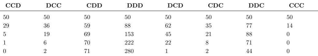
Starting with 50 of each of the eight player types, randomly paired, Table 3 shows how the player type counts evolve over a typical ten round tournament. Our previous examination of Table 2 has prepared us for the results: after 10 rounds, all surviving players are playing “defect” every move of every game. The average payoff per player has fallen to 1.

Table 3: Player Type Counts by Round

CCD DCC CDD DDD DCD CDC DDC CCC

50 50 50 50 50 50 50 50

29 36 59 88 62 35 77 14

5 19 69 153 45 21 88 0

1 6 70 222 22 8 71 0

0 2 71 280 1 2 44 0

17

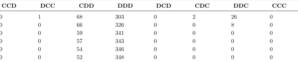
Table 3: Player Type Counts by Round

CCD DCC CDD DDD DCD CDC DDC CCC

0 1 68 303 0 2 26 0

0 0 66 326 0 0 8 0

0 0 59 341 0 0 0 0

0 0 57 343 0 0 0 0

0 0 54 346 0 0 0 0

0 0 52 348 0 0 0 0

7

Evolutionary Grid

The evolutionary prisoner’s dilemma is often played on a grid, which simplifies exploring the implications for player type evolution of various characterizations of the neighborhood in which a player resides.18

In this section we make use of a grid that is torus-like (in that it wraps around its edges), and we define the neighborhood of a player to include the player above, the player below, and the player to each side.19

Each player has a fixed location on the grid. This means that every player has the same four neighbors throughout a tournament, although the player types of these players can of course evolve over time.

The implementation of an evolutionary grid profits substantially from our earlier work at representing players, games, rounds, and tournaments. The code in thesimple_grid.pylisting is all we need to add (aside from a grid object with aget_neighborsmethod, which is provided in theuser_utils module---see the appendix). A GridPlayer inherits almost all its behavior from SoupPlayer: A GridPlayer

is just a SoupPlayer that has a grid that knows know how to determine its neighbors. Similarly, the only thing we need to do to produce a GridRound is inherit from SimpleRound and over-ride therun

definition. Even the run method is very modestly changed: in effect a player now has more than one neighbor, and correspondingly plays aCDIGameonce with each neighbor. Recall that a player will know which games it has played, because itsgames_playedattribute is appended when aCDIGameis run.

# L i s t i n g : s i m p l e g r i d . py

from s i m p l e s o u p import ∗

c l a s s G r i d P l a y e r ( SoupPlayer ) :

d e f g e t n e i g h b o r s ( s e l f ) : #d e l e g a t e t o t h e g r i d r e t u r n s e l f . g r i d . g e t n e i g h b o r s ( s e l f )

c l a s s GridRound ( SimpleRound ) : d e f run ( s e l f ) :

s e l f . p r e p a r e p l a y e r s ( ) f o r p l a y e r i n s e l f . p l a y e r s :

n e i g h b o r s = p l a y e r . g e t n e i g h b o r s ( ) f o r n e i g h b o r i n n e i g h b o r s :

i f n e i g h b o r not i n p l a y e r . p l a y e r s p l a y e d : game = CDIGame( p l a y e r , n e i g h b o r ) game . run ( )

p a y o f f s = game . p a y o f f ( ) s e l f . e v o l v e p l a y e r s ( )

18

It is not always appreciated that a two-dimensional grid is just a convenient and intuitive conceptualization of rela-tionships that are easily characterized in terms of a one-dimensional array. The class implementing the grid therefore need not rely on any kind of two-dimensional container object, although the class we provide as a user utility (see the appendix) does in fact do so: lists of lists provide fast and convenient access. (Users of thenumpymodule might instead consider using object arrays, which offer numpy’s powerful indexing facilities.)

19

This is known as the von Neumann neighborhood of radius 1, where a von Neumann neighborhood of radiusr

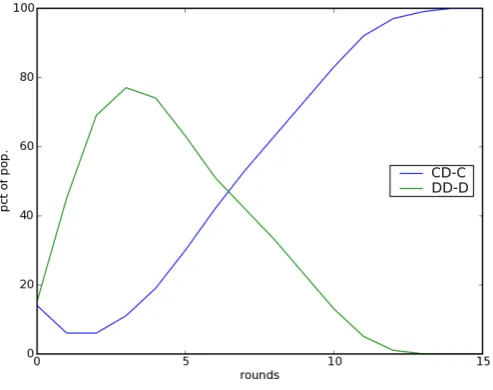
The result of running such a tournament has often been viewed as surprising and interesting. [axelrod hamilton-1981scien note that the “Tit-for-Tat” strategy (CD-C) is very robust in such settings, and indeed we find that it

often squeezes out all other strategies. Figure 1 summarizes a typical tournament. (Only two of the eight player types are plotted.)

Figure 1: Evolving Strategy Frequencies: Evolutionary Grid

We can understand the success of the CD-C strategy that we see in Table 4 in terms of our results in Table 2. Consider two adjacent CD-C players on a grid that is otherwise entirely populated by DD-D players. Using the notation of [rapoport chammah-1965], let the payoff matrix be represented symbolically as[[(R,R),(S,T)],[(T,S),(P,P)].

Each of the two CD-C players will receive a payoff of R+3S from its first move (summed across all 4 neighbors) and a payoff of R+3P from its second and subsequent moves (summed across all 4 neighbors). Given a 4 move game, that is a total payoff of 4R+9P. In contrast a DD-D player who has a CD-C player as a neighbor will receive a payoff of T+3P from its first move (summed across all 4 neighbors). and a payoff of 4P for each move thereafter (summed across all 4 neighbors). Given a 4 move game, that is a total payoff of T+15P. So the CD-C type players get a higher payoff as long as 4R+3S>T+6P.

In the literature it is common to let each game run for at least 4 moves. Using the canonical prisoner’s dilemma payoffs,[[(R,R),(S,T)],[(T,S),(P,P)]=[[(3,3),(0,5)],[(5,0),(1,1)]. This means that the highest average payoff will go to the CD-C players. (The two CD-C players in this case each receive a payoff of 21, while a DD-D neighbor will receive 20.) The neighboring DD-D players will therefore switch strategies (with probability determined by the selection pressure) thereby increasing the number of adjacent CD-C players. Naturally, the “Tit-for-Tat” strategy quickly takes over the grid!

Contrary to a common impression, this does not _{mean that CD-C is the best strategy on our}

evo-lutionary grid. Two obvious changes will make DD-D and CD-D win the evoevo-lutionary race. First, we could reduce the number of moves in each game to 3. (The two CD-C players in this case each receive a payoff of 3R+6P=15, while a DD-D neighbor will receive T+11P=16.) Alternatively, we could deviate from the canonical payoff matrix we have been using.

We will explore the second possibility. To keep the discussion focused, we will focus on a single parameter: P. Consider for example raising the value of P, retaining the canonical payoffs T=5, S=0, and R=3. Recall our isolated CD-C pair will beat their DD-D neighbors as long as 4R+9P+3S>T+15P: that is, as long as 7/6>P. If we raise P above this threshold, then the DD-D neighbors will win and the CD-C pair will switch strategies. Intuitively, if we reduce the punishment defection of defection, we expect defection to be more likely to persist as a strategy [rapoport chammah-1965].

Each of the four CD-C players has two CD-C neighbors and two DD-D neighbors. Each therefore receives a payoff of 8R+6P+2S (one round, four moves per game). The neighboring DD-Ds each get a payoff of T+15P. The CD-Cs have the better payoff if 8R+6P+2S>T+15P. Again retaining T=5, R=3, and S=0, this means that as long as 19/9>P the CD-C players will have the higher payoff. All the DD-D neighbors will thereafter adopt CD-C strategies, and this expansion will continue outward from the initial square.

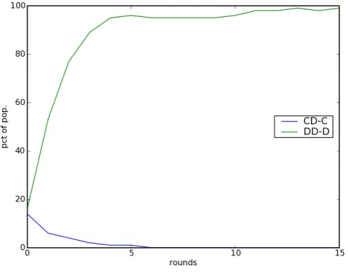
In more general terms, as we raise the payoff to mutual defection, it becomes harder and harder for the CD-C strategy to win out over the DD-D strategy on our evolutionary grid. The canonical payoff matrix makes it almost inevitable the the CD-C player type will come to dominate the grid. As we raise the value of P high enough, it becomes almost inevitable for the DD-D player type to come to dominate the grid. This happens relatively soon: for the payoff matrix [[(3,3),(0,5)],[(5,0),(1.8,1.8)]], the outcome in Figure 2 is rather typical.

Figure 2: Evolution of Player Types: Less Punishment of Mutual Defection

8

Commitment

We have seen that, with a standard grid topology for an evolutionary iterated prisoner’s dilemma, cardinal aspects of the payoff matrix affect the likelihood that a random mix of player types will evolve toward defection or cooperation. We now consider an additional influence on this outcome: commitment, considered as an unwillingness to imitate the strategies of others.

As a tentative application, consider software patents. Some software manufacturers and some re-searchers contend that the recent explosion of software patenting can damage software productivity---for example, by creating patent thickets. (See [isaac park04 colombatto] for an extensive discussion.) The United States appears particularly susceptible to such problems: both manufacturers and researchers have argued that nonobviousness requirements are not being enforced by the US Patent and Trademark Office. Some firms have responded to the situation by asserting that they will not enforce certain collec-tions of patent claims except in retaliation for patent claims against them. This may improve aggregate productivity and overall industry profits by increasing knowledge flows and reducing litigation costs, but at the individual firm level the temptation to defect will be present. Some firms, most famously IBM, have responded to this situation by publically a commitment not to “defect”.

# L i s t i n g : c o m m i t p l a y e r . py

from s i m p l e g r i d import ∗

c l a s s CGridPlayer ( G r i d P l a y e r ) : p commit = 0

d e f i n i t ( s e l f , p l a y e r t y p e ) :

G r i d P l a y e r . i n i t ( s e l f , p l a y e r t y p e ) i f p l a y e r t y p e . p == ( 0 , 1 , 0 ) :

s e l f . committed = random ( ) < s e l f . p commit e l s e :

s e l f . committed = F a l s e d e f e v o l v e ( s e l f ) :

i f not s e l f . committed and random ( ) < s e l f . s e l e c t i o n p r e s s u r e : s e l f . p l a y e r t y p e = s e l f . n e x t p l a y e r t y p e

TheCGridPlayer class is defined so that instances behave identically toGridPlayerinstances: the class variable p_commit is assigned a value of 0 in the class definition. However this behavior can be changed by assigning new values to p_commit. Intuition suggests that the existence on the grid of committed Tit-for-Tat players makes it more likely that a high payoff cluster of Tit-for-Tat players can form during the tournament.20

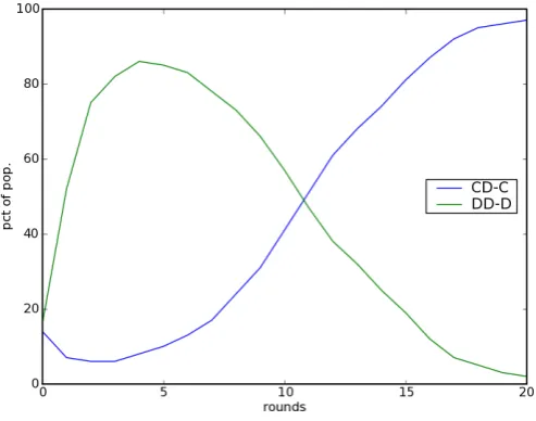
An illustrative verification of this intuition is offered in Figure 3, which shows the concentration of DD-D and CD-C players over time when the probability of a CD-C player committing is 0.2. The outcomes closely resemble Figure 1 even though the payoffs are those used in producing Figure 2. Holding all other aspects of the game are constant across the two scenarios, but leavingp_commit=0, produces a outcome closely resembling Figure 2. The presence of committed players radically alters the evolution of playertypes.

Figure 3: Evolution of Player Types: With Committed Players

Naturally this verification of our intuition is only illustrative. The initial configuration of players on the grid is random, and a given value of p_commit cannot tip the balance for all distributions. (For example, even a high probability that Tit-for-Tat players are committed cannot help if chance dictates that there are few of them and they are each surrounded by players that will exploit them, such as DD-D players.) The important point, however, is that a modest probability of commitment can radically change the playertype evolution. Correspondingly, there is a change in the average payoff received by players on the grid. This may be considered a social consequence of commitment.

20

9

Conclusion

Researchers using computer simulation of economic interactions often promote ACE methods as a “third way” of doing social science, distinct from both pure theory and from statistical exploration [axelrod1997abm]. One hope of ACE researchers is that unexpected but useful (for prediction or under-standing) aggregate outcomes will “emerge” from the interactions of autonomous actors. The iterated prisoner’s dilemma is a good illustration of the fruition of this hope: more than two decades of compu-tational exploration have delivered many interesting and surprising results. Classic among these is the high fitness of the “Tit-for-Tat” player type on an evolutionary grid.

This paper uses the iterated prisoner’s dilemma as a spring board for exposition and exploration. The paper demonstrates that useful ACE models can be constructed with surprising ease in a general purpose programming language, if that language has the flexibility and readability of Python. Python’s combination of compactness and readability means that a full listing of the code needed to produce the half dozen simulations described in this paper takes only a few pages.

The simulations presented accomplish several purposes. The initial simulations lay bare the under-pinnings of some classic results, demonstrating in the process the usefulness of an object approach to modeling IPDs. We then show that, by manipulating a single entry of the payoff matrix while remaining within the standard definition of the prisoner’s dilemma, payoff matrix values are crucial to outcomes on an evolutionary grid. This acts as a cautionary tale for those relying on the canonical payoffs for their simulations. Finally, we introduce a simple notion of commitment, and we find dramatic implications for the evolution of strategies over time. Paradoxically, although committed players do not imitate the most successful neighboring strategy, they may generate social outcomes that increase the payoffs for all players (including the committed players).

10

Appendix A

This appendix contains a small number of user utilities that were used to simplify the code samples in the main text.

# F i l e : u s e r u t i l s . py

from random import random , s h u f f l e

from random import c h o i c e a s randomchoice #a r e a d e r c o n v e n i e n c e import i t e r t o o l s

############################################################# ########### s i m p l e u t i l i t i e s ############################## #############################################################

d e f mean ( l s t ) : #s i m p l e s t computation o f mean n = l e n ( l s t )∗1 .

r e t u r n sum ( l s t ) / n

d e f t r a n s p o s e ( s e q s e q ) : #s i m p l e 2−d i m e n s i o n a l t r a n s p o s e r e t u r n z i p (∗s e q s e q )

d e f f i n d b e s t p l a y e r t y p e s ( p l a y e r s ) : #c a l l e d by SoupPlayer b e s t p l a y e r s = l i s t ( )

b e s t p a y o f f = −1e9 f o r p l a y e r i n p l a y e r s :

p a y o f f = p l a y e r . g e t p a y o f f ( ) i f p a y o f f == b e s t p a y o f f :

b e s t p l a y e r s . append ( p l a y e r ) i f p a y o f f > b e s t p a y o f f :

b e s t p a y o f f = p a y o f f b e s t p l a y e r s = [ p l a y e r ]

d e f c o u n t p l a y e r t y p e s ( p l a y e r s ) : #c a l l e d by SimpleTournament summary = d i c t ( ) #empty d i c t i o n a r y

f o r p l a y e r i n p l a y e r s :

ptype = p l a y e r . p l a y e r t y p e

summary [ ptype ] = summary . g e t ( ptype , 0 ) + 1 r e t u r n summary

d e f g r o u p s o f ( l s t , n ) : #used t o p o p u l a t e SimpleTorus by row

””” Return l e n ( s e l f ) / / n gr o up s o f n , d i s c a r d i n g l a s t l e n ( s e l f )%n p l a y e r s . ””” #u s e i t e r t o o l s t o a v o i d c r e a t i n g unneeded l i s t s

r e t u r n i t e r t o o l s . i z i p (∗[ i t e r ( l s t ) ]∗n )

############################################################# ############## v e r y s i m p l e g r i d c l a s s ###################### #############################################################

c l a s s SimpleTorus :

n e i g h b o r h o o d = [ ( 0 , 1 ) , ( 1 , 0 ) , ( 0 ,−1 ) , (−1 , 0 ) ] d e f i n i t ( s e l f , ( nrows , n c o l s ) ) :

s e l f . nrows = nrows s e l f . n c o l s = n c o l s

s e l f . n e i g h b o r s = d i c t ( ) #empty d i c t i o n a r y d e f p o p u l a t e ( s e l f , p l a y e r s ) :

s e l f . p l a y e r s = l i s t ( l i s t ( group ) f o r group i n g r o u p s o f ( p l a y e r s , s e l f . n c o l s ) f o r r i n r a n g e ( s e l f . nrows ) :

f o r c i n r a n g e ( s e l f . n c o l s ) : p l a y e r = s e l f . p l a y e r s [ r ] [ c ] p l a y e r . g r i d = s e l f

p l a y e r . l o c = r , c d e f g e t n e i g h b o r s ( s e l f , p l a y e r ) :

i f p l a y e r i n s e l f . n e i g h b o r s :

n e i g h b o r s = s e l f . n e i g h b o r s [ p l a y e r ] e l s e :

p l a y e r r o w , p l a y e r c o l = p l a y e r . l o c n e i g h b o r s = l i s t ( ) #empty l i s t f o r o f f s e t i n s e l f . n e i g h b o r h o o d :

dc , dr = o f f s e t #bc x , y n e i g h b o r h o o d r = ( p l a y e r r o w + dr ) % s e l f . nrows c = ( p l a y e r c o l + dc ) % s e l f . n c o l s n e i g h b o r = s e l f . p l a y e r s [ r ] [ c ] n e i g h b o r s . append ( n e i g h b o r ) r e t u r n n e i g h b o r s

11

References

[axelrod1997abm] Axelrod, Robert. 1997. The Complexity of Cooperation: Agent-Based Models of Competition and Collaboration.

[hahn1991ej] Hahn, Frank. 1991. The Next Hundred Years. ej 101, 47--50.

[bonabeau2002pnas] Bonabeau, Eric. 2002. Agent-based Modeling: Methods and Techniques for Simulating Human Systems. pnas 99, 7280--7.

[luna stefansson2000swarm] Luna, Francesco, and Benedikt Stefansson. 2000. Economic Simulations in {Swarm}: Agent-Based Modelling and Object Oriented Program-ming.

[kak2003oop] Kak, Avinash. 2003. Programming with Objects: A Comparative Pre-sentation of Object Oriented Programming with C++ and Java.

[matsumoto kurita-1998-acmt] Matsumoto, M, and Y Kurita. 1998. Mersene Twister: A 623-Dimensionally Equidistributed Uniform Pseudo-Random Number Gen-erator. ACM Transactions on Modeling and Computer Simulation 8, 3--30.

[poundstone1992] Poundstone, W. 1992. Prinsoner’s Dilemma.

[stefansson2000 luna stefansson] Stefansson, Benedikt. 2000. Simulating Economic Agents in{Swarm}.

[rapoport chammah-1965] Rapoport, Anatol, and Albert M Chammah. 1965. Prisoner’s Dilemma: A Study in Conflict and Cooperation.

[trivers-1971-qrbio] Trivers, Robert L. 1971. The Evolution of Reciprocal Altruism. Quar-terly Review of Biology 46, 35--57.

[axelrod hamilton-1981science] Axelrod, Robert, and William D Hamilton. 1981. The Evolution of Cooperation. Science 211, 1390--6.