Algorithm Tuning from Comparative Analysis of
Classification Algorithms
Thaung Myint Htun*, Zaw Tun**
*
Faculty of Information Science, University of Computer Studies, Sittway
**
Admin Office, University of Computer Studies, Sittway
DOI: 10.29322/IJSRP.8.5.2018.p7767
http://dx.doi.org/10.29322/IJSRP.8.5.2018.p7767
Abstract- Machine Learning is the upcoming research area to solve various problems and classification is one of main problems in the field of machine learning. This paper describes various Supervised Machine Learning (ML) classification techniques, compares various supervised learning algorithms as well as determines the most efficient classification algorithm based on the dataset. Wine-quality-white dataset is taken from UCI machine learning repository. Six different machine learning algorithms are considered: Logistic Regression (LR), Linear Discriminant Analysis (LDA), K-Nearest Neighbors (KNN), Classification and Regression Trees (CART), Gaussian Naïve Bayes (NB) and Support Vector Machine (SVM). By tuning of neighbors for KNN,the best configuration is K= 1.
Index Terms- Accuracy, Algorithm Tuning, Classification, Machine Learning.
I. INTRODUCTION
achine learning is a paradigm that may refer to learning from past experience to improve future performance. Learning refers to modification or improvement of algorithm based on past “experiences” automatically without any external assistance from human[3].
Bill Gates, Former Chairman, Microsoft said that a breakthrough in machine learning would be worth ten Microsofts. Machine learning (ML) is getting computers to program themselves. ML is like farming or gardening. Seed is the algorithm, nutrient is the data, the gardeners are like us and plant in the program. If programming is automation, then machine learning is automating the process of automation. Writing software is bottleneck, we don’t have enough good developers. Let the data do the work instead of people. Machine learning is the way to make programming scalable.
Machine learning aims to generate classifying expressions simple enough to be understood easily by the human. They must mimic human reasoning sufficiently to provide insight into the decision process. Like statistical approaches, background knowledge may be exploited in development, but operation is assumed without human intervention [2].
Machine learning techniques are used for data analysis and pattern discovery. Thus play a major role in the development of data mining applications [6]. There are many different methods to compare results and to determine the best classification.
Machine learning is concerned with techniques and algorithms for performing tasks that improve with experience at performing specific tasks [1]. The main categories of machine learning tasks are classification, regression, clustering, co-training, relationship discovery, and reinforcement learning.
II. WINE-QUALITY CLASSIFICATION 2.1 Wine-quality-white dataset
Wine-quality dataset is taken from real data. There are 11 attributes and 7 classes. All attributes are numeric-valued. The 11 attributes are fixed acidity, volatile acidity, citric acid, residual sugar, chlorides, free sulfur dioxide, total sulfur dioxide, density, pH, sulphates and alcohol.
2.2 Supervised machine learning procedure
One standard formulation of the supervised learning task is the classification problem. Inductive machine learning is the process of learning a set of rules from instances, or more generally speaking, creating a classifier that can be used to generalized from new instances.
The process of applying supervised ML to a real-world problem is described in Figure 1.
This work focuses on the classification of ML algorithms and determining the most efficient algorithm with highest accuracy and precision.
2.3 Classification comparison procedure:
Algorithms compared use same wine quality-white dataset (11 attributes and 7 classes) in order to have fair comparison result. One attribute (class) is set as output (target) while the others as input to algorithms.
There are several steps be done for this comparison:
1. simulate each algorithm by using all attribute dataset and find the best setting to get highest accuracy for each algorithm. Referred as all attributes.
2. Feature selection by removing an attribute, and re simulate for each algorithm. Referred as reduced attributes.
3. Eliminate the worst class recall of the best algorithm found at step 2, and re simulate only for the best algorithm.
III. METHODOLOGY 3.1 Measuring the Central Tendency
Descriptive statistics can give us great insight into the shape of each attribute.
Mean: The common and most effective numerical measure of the center of a set of data is the (arithmetic) mean.
kth Percentile: The kth percentile of a set of data in numerical order is the value xi having the property that k percent of the
data entries lies at or below xi . The median is the 50th percentile.
The first quartile, denoted by Q1, is the 25th percentile; and the third quartile, denoted by Q3, is the 75th percentile.
Standard Deviation: It is measures of data dispersion. It indicates how spread out a data distribution is. A low standard deviation means that the data observations tend to be very close to the mean, while a high standard deviation indicates that the data are spread out over a large range of values.
Max-Min Normalization: It performs a linear transformation on the original data. Suppose that minA and maxA are the minimum
and maximum value of an attribute, A.
3.2 Learning Algorithms
Naïve Bayes: A naïve bayes classifier is based on the Bayes theorem. A naive bayes classifier is based on the Bayes theorem. A naïve bayes classifier assumes that the presence of an articular feature of a class is unrelated to the presence of any other feature (input variable is independent).
Naïve bayes classification can be trained very efficiently in a supervised learning setting. Parameter estimation for naïve bayes uses the method of maximum likelihood or using bayesian methods.
The assumption that input variable is independent is unrealistic for real data. This technique is very effective on a large range of complex problems [5].
Support Vector Machine(SVM): SVM is categorized as supervised learning which considered as heuristic algorithm. The main idea in SVM is to determine a hyper plan that optimally separates two classes.
Kernel function is used to solve classification function. There are four basic kernels functions [5]:
- Linear : K(xi, xj) = xiTxj
- Polynomial : K(xi, xj) = (yxi Txj+ r)d, y> 0
- RBF : K(xi, xj) = exp(-yǁ xi - xjǁ2), y>0
- Sigmoid : K(xi, xj) = tanh(yxi Txj+ r)
RBF is radial basis function. The y, r, and d are kernel parameters. In this paper, Linear Function is used as the kernel function in order to get better accuracy.
k-Nearest Neighbors (KNN) :This algorithm, also known as
“lazy learning algorithm” is the simplest algorithm of all the machine learning models. It compares a given example ’x’ with training examples which are similar to it.
The training dataset is stored in a n-dimensional pattern space and the algorithm searches the area for the nearest example (k) from the training dataset that is close to the given example x. This algorithm usually is used for classification and regression. Regarding classification, it classifies according to the majority vote of it is nearest k. K is a positive integer. When k = 1, this means it is assigned to the nearest neighbor.
Decision Tree: The representation of decision tree model is a binary tree. Each node represents a single input variable (x) and a split on that variable. The leaf nodes of the tree contain an output variable (y) which is used to make a prediction. Predictions are made by walking the split of the tree until arriving at a leaf node and output the class at that leaf node.
Trees are fast to learn and very fast for making predictions. Decision Tree is also accurate for a broad range of problems and do not require any special preparation for data. Decision Tree has a high variance and can yield more accurate predictions when used in an ensemble.
Logistic Regression(LR): Linear regression can easily be used for classification in domains with numeric attributes. Indeed, we can use anyregression technique, whether linear or nonlinear, for classification. The trick is to perform a regression for each class, setting the output equal to one for training instances that belong to the class and zero for those that do not. The result is a linear expression for the class. Then, given a test example of unknown class, calculate the value of each linear expression and choose the one that is largest. This method is sometimes called multi-response linear regression.
Linear Discriminant Analysis: Linear Discriminant Analysis (LDA) is a statistical technique for binary and multiclass classification. It too assumes a Gaussian distribution for the numerical input variables. LR and LDA are simple linear algorithms.
3.3 Algorithm Tuning
algorithm. The objective of algorithm tuning is to find the best point or points in that hypercube for our problem. We will be optimizing against our test harness, so again we cannot underestimate the importance of spending the time to build a trusted test harness.
Algorithm parameter tuning is an important step for improving algorithm performance right before presenting results or preparing a system for production.
IV. RESULTS
We use scikit-learn from Python to explore the data both with descriptive statistics and data visualization. We must have a very good handle on how much data we have, both in terms of rows and columns. Too many rows and algorithms may take too long to train. Too few and perhaps we do not have enough data to train the algorithms. Too many features and some algorithms can be distracted or suffer poor performance due to the curse of dimensionality.
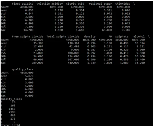
[image:3.612.314.572.61.205.2]We can take a look at a summary of each attribute at Figure 1. This includes the count, mean, the min and max values as well as some percentiles.
Figure 1. Reviewing statistical summary of data and class distribution in the dataset
We can view the number of instances that belong to each class. We can present a histogram of each input variable at Figure 2. We can view that there are Gaussian-like distributions and perhaps some exponential like distributions for other attributes. We can present same perspective of the data using density plots in Figure 3.
[image:3.612.315.574.249.378.2]This is useful, we can view that many of the attributes have a skewed distribution. A power transform like a Box-Cox transform that can correct for the skew in distributions might be useful.
[image:3.612.35.300.325.541.2]Figure 2. Histogram Plots of Attributes from the Dataset
Figure 3. Density Plots of Attributes from the Dataset
4.1 Correlations Between Attributes
Correlation gives an indication of how related the changes are between two variables. If two variables change in the same direction they are positively correlated. If they change in oppositely directions together, then they are negatively correlated.
We can plot the correlation matrix and get an idea of which variables have a high correlation with each other. We can also see that each variable is perfectly positively correlated with each other in the diagonal line from top left to bottom right as shown in Figure 4.
[image:3.612.316.569.524.717.2]4.2 Evaluation Algorithms : Basedline
We don’t know what algorithms will do well on Wine-quality-white dataset. Gut feel suggests distance based algorithms like k-Nearest Neighbors and Support Vector Machines may do well. We use 10-fold cross-validation. The dataset is not too small and this is a good standard test harness configuration. We evaluate algorithms using the accuracy metric. This is a gross metric that give a quick idea of how correct a given model is. Table 1 shows the accuracy result for each model.
We create a baseline of performance on this paper and spot-check a number of different algorithms. We select a suite of different algorithms capable of working on this classification research. The six algorithms selected include:
• Linear Algorithms: Logistic Regression (LR) and
Linear Discriminant Analysis (LDA).
[image:4.612.356.527.217.412.2]• Nonlinear Algorithms: Classification and Regression Trees (CART), Support Vector Machine (SVM), Gaussian Naïve Bayes (NB) and k-Nearest Neighbors (KNN).
Table 1. Accuracy Result for Each Model
Model Accuracy Score
LR 0.522722
LDA 0.525787
KNN 0.466297
CART 0.588051
NB 0.441816
SVM 0.5564
[image:4.612.68.239.257.474.2]There are just mean accuracy values. It is always wise to look at the distribution of accuracy values calculated across-validation folds. We can present that graphically using box and whisker plots in Figure 5.
Figure 5. Box and Whisker Plots of Algorithm Performance
4.3 Evaluation Algorithms : Standardize Data
We evaluate the same algorithms with a standardized copy of the dataset. This is where the data is transformed such that each attribute has a mean value of zero and a standard deviation of one. We also need to avoid data leakage when we transform the data.
A good way to avoid leakage is to use pipelines that standardize the data and build the model for each fold in the cross-validation test harness. That way we can get a fair estimation of how each model with standardized data might perform on unseen data. Table 2 describes the accuracy result for each standardized model.
Table 2. Output of Evaluating Algorithms on Standardized Dataset
Model Accuracy Score
Scaled LR 0.528338
Scaled LDA 0.525787
Scaled KNN 0.550532
Scaled CART 0.589077
Scaled NB 0.439774
Scaled SVM 0.563555
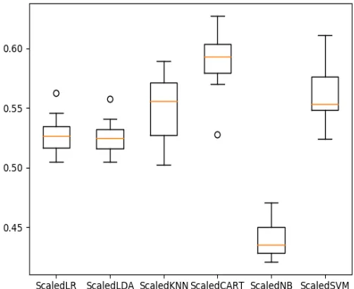
[image:4.612.313.564.463.668.2]We plot the distribution of the accuracy scores using box and whisker plots in Figure 6.
[image:4.612.45.285.538.723.2]4.4 Algorithm Tuning
According to Table 1, the results show a tight distribution for CART and SVM are encouraging, suggesting low variance. The poor results for KNN and NB are surprising. According to Table2, we can see that SVM, CART are still doing well, even better than before.
We tried to research digging deeper into the SVM and KNN algorithms. It is very likely that configuration beyond the default may yield even more accurate models.
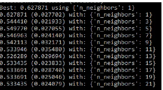
We can start off by tuning the number of neighbors for KNN. The default number of neighbors is 7. Below we tried all odd values of k from 1 to21, covering the default value of 7. Each k value is evaluated using 10- fold cross-validation on the training standardized dataset.
We can print out configuration that resulted in the highest accuracy as well as the accuracy of all values tried as shown in Figure 7.
Figure 7.Result of Tuning KNN on the Standardized Dataset
We can tune two key parameters of the SVM algorithm, the value of C (how much to relax the margin) and the type kernel. The default for SVM is to use the Radial Basis Function (RBF) kernel with a C value set to 1.0. Like with KNN, we will perform a grid search using 10-fold cross-validation with a standardized copy of the training dataset. We tried a number simpler kernel types and C values with less bias and more bias. The accuracy 64.954 % is better than what KNN and CART could achieve.
V. CONCLUSION AND RECOMMENDATION
We worked through a classification predictive modeling in machine learning. We have met our objective which is to
evaluate and investigate six selected classification algorithms. The best algorithm based on the data is SVM according to algorithm tuning. In Tuning, k=1 for KNN was good, SVM with accuracy 64.954% was the best.
Machine Learning classification requires thorough fine tuning of the parameters and at the same time sizeable number of instances for the dataset. It is not a matter of time to build the model for the algorithm only but precision and correct classification. Therefore, the best learning algorithm for a particular data set does not guarantee the precision and accuracy for another set of data whose attribute are logically different from the other[4]. This work recommends that we can improve the performance of algorithms by using ensemble methods. Then we can finalize the model by training it on the entire training dataset and make predictions for the hold-out validation dataset to confirm our findings.
REFERENCES
[1] Claire Gallagher, Michael G. Madden, Brian D.Arcy, “A Bayesian Classification Approach to Improving Performance for a Real-World Sales Forecasting Application”
[2] Danal. Michie, D.J. Spiegelhalter, C.C. Taylor, “Machine Learning, Neural and Statistical Classification”, 17-February-1994, pp-6-20,107-109 [3] Kajaree Das, Rabi Narayan Behera, A Survey on Machine Learning:
Concept, Algorithms and Applications.
[4] Neocleous C. & Schizas C. (2002). Artificial Neural Network Learning: A Comparative Review. In: Vlahavas I.P., Spyropoulos C.D. (eds)Methods and Applications of Artificial Intelligence. Hellenic Conference on Artificial Intelligence SETN 2002. Lecture notes in Computer Science, Volume 2308. Springer, Berlin, Heidelberg, doi: 10.1007/3.540-46014-4_27 pp. 300-313. Available at: https://link.springer.com/chapter/10.1007/3-540-46014-4_27 [5] Pramudyana Agus Harlianto, N.A.Setiawan and T.B.Adji, “Comparison of
Machine Learning Algorithms for Soil Type Classification”
[6] Swe Swe Aung, Itaru Nagayama, Shiro Tamaki, “Correlation Coefficient-based K-means Clustering for K-NN”, Yangon, 16-17 February 2017
AUTHORS
First Author – Thaung Myint Htun , Ph.D Candicate, University of Computer Studies, Sittway, Myanmar, [email protected]
Second Author – Zaw Tun, Ph.D,
[image:5.612.39.299.261.405.2]