Ant Colony Accumulative Technique Applied in Wireless
Sensor Network Grids Routing Problem
Ashraf Hussein
Operation Research CenterEgypt.Cairo Helwan University
Mostafa Sami
Manger of Computer scienceDepartment Egypt.Cairo Helwan University
Hisham Dahshan
Communication TeacherEgypt.Cairo Military Technical College
ABSTRACT
This contribution presents a proposal of an applicable routing messages protocol (RMP) which uses nodes location information and a multi-hop forwarding scheme to achieve long-range communication in Wireless Sensor Network Grids (WSNG). Ant Colony (ACO) accumulative technique has been applied to collect the hops list in the message way toward the sink. The proposed RMP has three phases: firstly, the initialization phase where each sensor node determines the best first hop toward the Sink among its neighbors. Secondly, sending the best route phase where each node sends an accumulative routing message (ARM) to the sink includes the hops list. Thirdly, in the maintenance phase, the out of reach node sends a maintenance accumulative routing message (MARM) to create the alternative route to the Sink. The proposed RMP provides a simple and applicable routing model for WSNG. It also makes the total energy consumed in data transmission more efficient in the sensor network and minimizes the node memory size and processing steps which reduces the total network cost.
General Terms
Wireless sensor network Grids, Ant Colony.
Keywords
Sink, Sensor node.
1.
INTRODUCTION
Wireless grid architectures can be classified into four categories based on the devices predominant in the grid and the relative mobility of the devices in the grid: Fixed Wireless Grids, Mobile or Dynamic Wireless Grids, Ad Hoc grids and Wireless Sensor Network Grids [5].WSNG consists of a large number of sensor nodes densely deployed either close to or inside a phenomenon. These nodes are distributed randomly, self-organized, have cooperative capabilities, prone to failures, network topology changes frequently [1, 2], limited in power, have limited memory capacities, and limited cost for each node [3, 4]. The main function of a WSNG is to sense and report events which can only be meaningfully if the accurate location of the event is known. Gathering and transmitting the sensed data to the base station needs to be accomplished to meet the end-user queries. Designing an efficient routing scheme that can collect massive data and offer good performance in energy efficiency is important to the network life time. This work propose a multi-hop forwarding routing messages protocol (RMP) using ant
colony accumulative technique to achieve long-range communication. The paper is organized as follows: Section 2 introduces a brief explanation of the ACO. Section 3 presents related work. The proposed routing message protocol (RMP) is presented in Section 4. Mathematical Analysis of the proposed scheme is presented in Section 5. The performance evaluation of the proposed scheme is presented in Section 6. Finally, Sections 7 concludes the paper.
2.
ACO
ACO is an algorithm that utilizes the behavior of the real ants in finding a shortest path from a source to the food [13, 15, and 16]. It has been observed that the ants deposit a certain amount of pheromone in its path while traveling from its nest to the food. Again while returning, the ants are subjected to follow the same path marked by the pheromone deposit and again deposit the pheromone in its path. In this way the ants following the shorter path are expected to return earlier and hence increase the amount of pheromone deposit in its path at a faster rate than the ants following a longer path. However, the pheromone is subjected to evaporation by a certain amount at a constant rate after a certain interval. Therefore, the paths visited by the ants frequently, are only kept as marked by the pheromone deposit, whereas the paths rarely visited by the ants are lost due to the lack of pheromone deposit on that path. Consequently, the new ants are intended to follow the frequently used paths only. Thus, all the ants starting their journey can learn from the information left by the previously visitor ants and are guided to follow the shorter path directed by the pheromone deposit. In ACO, a number of artificial ants (here data packets) build solutions to the considered optimization problem at hand. They also exchange information on the quality of these solutions via a communication scheme that is pheromone deposit on the path of the journey performed by it.
3.
Related work
at a dissemination node is forward along the reverse grid path of the advertisement to the data source, and then the requested data is returned along the same path to the requesting node. Simple geographic forwarding is used to move messages between dissemination nodes on the grid. The grid structure used by TTDD efficiently overcomes the problem encountered by geographic routing when irregularly-shaped holes exist in the sensor field caused by sensor failure or the random deployment.
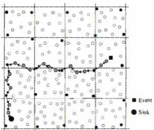
J. Homsberger and G. C. Shoja have addressed a different grid structure routing protocol with TTDD. Their proposed scheme is called the Geographic Grid Routing (GGR) protocol [10]. The GGR protocol is a hierarchical protocol for disseminating tasks in a sensor network and retrieving the corresponding data. The effort is broken into three stages; task dissemination, data forwarding and maintenance stage. The routing path of a message from the source to the sink after detecting an event by the source is shown in Figure 1.
Fig 1
:
The routing path in GGRChiu-Kuo Liang et al [11] present Steiner Trees Grid Routing STGR Protocol in order to reduce the total energy consumption for data transmission between the source node and the sink node. They construct a different virtual grid structure instead of the virtual grid introduced in GGR. Their idea is to construct the virtual grid structure based on the square Steiner trees as shown in Figure 2. It is to the best of author's knowledge; this algorithm presented in [11] is the recent work that addresses the specific location based model with respect to the WSNGs.
Fig 2
:
The routing path in STGR4.
The Proposed RMP
Let us assume the following characteristics: The sensor field is made up of hundreds or thousands of small, limited battery power and cheap sensing devices that are randomly deployed all through a two dimensional area of interest. Short-range radios with static transmission power are used due to the energy constraint. Therefore, multi-hop forwarding schemes are used to achieve long-range communication. The sensor nodes are assumed to have known location within the sensor field. An immobile data sink is deployed with the area of interest, and has location knowledge and an infinite power source. The proposed routing algorithm will be accomplished in three phases:
4.1
Phase I: (Initialization Phase)
Once the sensor nodes (SN) are deployed randomly, each sensor node in the network should have the location and ID of the fixed sink. Each sensor node starts to send a message containing its id and its location to all its neighbors that lie in its communication range. Then starts to determine the best 1st hop node toward the sink by calculating two distances D1 and D2 (D1 is the distance between each neighbor node and the sink), (D2 is the distance between each neighboring node and itself). Then calculate A which is equal to (d2-d1).
Each node chooses the best 1st hop node that has the largest A among its neighbors, as shown in the example in Fig 3. The best 1st hop for Sn1 is Sn5, Fig 4 illustrates the selective algorithm of phase I in RMP, notice that the for loop enables the node to apply the selective condition on its neighbors and come out with the best 1st hop ID. Notice that SA is a sensor node, N(sA) is a set of the neighbor nodes in the range, SJ is a sensor belongs to N(sA) and KJ is the sink node.
Fig 3
:
Example of applying the selective condition in RMP4.2
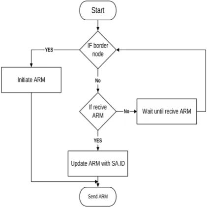
Phase II (ARM Phase):
By finishing phase I, each node at the edge of the network start to send an artificial ant (ARM ant) to the sink through the best nodes which has been determined in phase I. While the ARM ant travels hop by hop, it carries the ID of each intermediate node that it passes through until it reaches the sink.
[image:2.595.87.247.277.411.2] [image:2.595.318.538.420.524.2] [image:2.595.73.265.558.700.2]Start
z=0
d1(SJ) = |SJ,kJ| , d2(SJ) = |SJ,SA| A= (d2-d1)
If A > Z
z=A
SJN(SA)
forloop
End For loop
The best 1st hop ID= SJ.ID
No
End
Fig
4: the selective algorithm of phase I in RMPSn ID Inverse ARM
SN1 Sn109,Sn61,Sn54,Sn32,Sn7
SN7 Sn109,Sn61,Sn54,Sn32
SN32 Sn109,Sn61,Sn54
SN54 Sn109,Sn61
[image:3.595.54.275.60.741.2]SN61 Sn109
Fig 5: Example of the ARM message and the inverse ARM table
Start
If recive ARM
Update ARM with SA.ID
Send ARM
IF border node
Initiate ARM
Wait until recive ARM
No YES
No
[image:3.595.321.532.72.283.2]YES
Fig 6: Algorithm of phase II in RMP
4.3
Phase III (Maintaining the ARM table)
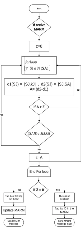
Each SN will count the number of completed communication session with the Sink, if it is smaller than certain thresholds it starts to send Maintenance artificial ant called MARM ant to recover the failure nodes that may defect the path as shown in the 1st algorithm in Figure 7. In the way of the MARM ant, each node receives MARM ant chose again the best 1st hop from all its neighboring nodes except the node it received MARM ant from or the node that has an ID included in the MARM unless it is the only choice. In the only choice case, the node flags it’s ID in the MARM ant and sends the MARM ant back to the last un-flagged node in MARM ant. When the MARM reaches the sink, the sink updates the ARM table using the inverse of the MARM ant, as shown in the 2nd algorithm in Figure 8.
Start
If the number of failed sessions > threshold
End No
Yes if the node recive a message & couldent reach the best 1st hop
Send MARM
resend the message go back one node
Yes
[image:3.595.53.270.395.729.2]send the message No
[image:3.595.318.506.487.732.2]Start
z=0
d1(SJ) = |SJ,kJ| , d2(SJ) = |SJ,SA| A= (d2-d1)
If A > Z
z=A
SJN(SA)
forloop
End For loop
The best 1st hop ID= SJ.ID Send MARM messege No If recive MARM MARM ID
ifSJ.
Yes
No
Update MARM
If Z = 0
There is no neighbor
Send MARM messege back flag its ID in the
[image:4.595.73.244.69.553.2]MARM Yes No
Fig 8: 2nd algorithm of phase III in RMP
4.4
ARM & MARM ants communication
overhead
ARM message which act as an artificial ant will have the following attributes; source ID, next hop ID, Sink ID, reported message and ARM sequence as shown in Figure 9.a. MARM message will have the following attributes; source ID, next hop ID, Sink ID, reported message, MARM sequence and Flagged IDs, as shown in Figure 9.b. Notice that the length of the ARM sequence and MARM sequence will be 2z bytes where z is the maximum number of hops toward the sink, while the length of flagged IDs will be 2x where x < z, x and z will be calculated in setup process depending on the following factors; the dimensions of the network area, the node communication range and the nodes distribution density.
[image:4.595.314.550.70.204.2]Source ID Next hop ID Sink ID Reported message ARM sequence 2 bytes 2 bytes 2bytes 8bytes 2z bytes
Fig 9a: ARM overhead structure
Source ID Next hop ID Sink ID Reported message MARM sequence Flagged IDs 2 bytes 2 bytes 2 bytes 8 bytes 2z bytes 2x bytes
Fig. 9b. MARM overhead structure
4.5
The proposed node memory structure
The node memory will have the following attributes; node ID, source ID, Sink ID, 1st hop ID, checked neighbor ID, distance D1, distance D2, calculated A, compared A, reported message, Sink location, node location , selected neighbor location, ARM sequence, MARM sequence and flagged IDs as shown in Figure 10. Notice that the proposed structure use Global Positioning System Fix Data location format which is one of the National Marine Electronics Association (NMEA) Global positioning system (GPS) standard format, which provide essential fix data for 3D location and accuracy data [12]. Node ID Source ID Next hop ID Sink ID checked neighbor ID Reported message 2 bytes 2 bytes 2 bytes 2 bytes 2 bytes 8 bytes ARM sequence MARM sequence Flagged IDs distance d1 distance d2 2z bytes 2z bytes
2x bytes 4 Bytes 4 bytes calculated A compared A Sink location node location selected neighbor location 4 bytes 4 bytes NMEA GPS format 64 bytes NMEA GPS format 64 bytes NMEA GPS format 64 bytes
Fig 10: The proposed node memory structure
5.
Mathematical Analysis of RMP
WSN consisting of n sensor nodes s1, s2... sn and m sinks k1, k2… km. The network can be modeled as an undirected graph G = (V, E), with the set of vertices V = v1 ∪ v2, with v1 being the set of SNs and v2 being the set of sinks. E is the set of edges. An edge exists between any two nodes that are in each other’s communication range. The set of vertices V = v1
∪ v2. Here, v1 = {s1, s2… sn} and v2 = {k1, k2… km} where n and m are system dependant parameters and represent the number of SNs and sinks respectively.
[image:4.595.311.549.363.563.2]equal values represent shortest D1 the best 1st hop will be the one which has the longest D2. Therefore, the equations below give the necessary conditions for determining the best 1st hop:
∀ [SA∈V1, kJ∈V2, SJ∈ N (SA)] there is D1 (SJ) = |SJ, kJ|, D2 (SJ) = |SJ, SA|
A= (D2 (SJ) - D1 (SJ)) & A is the largest number ∀ (N (SA))
6.
Performance Evaluation
The Performance evaluation focuses on the comparison of energy-efficient feature and the number of transmission hops between the proposed RMP, STGR and GGR protocols.
6.1
Simulation Environment
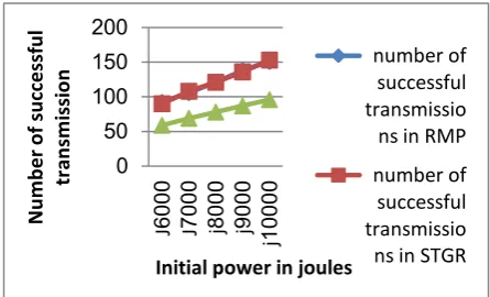
The authors built their own RMP simulation using object oriented software to enable us achieving the following stages: First, study area selection stage, which covers a subset of satellite image with its real Universal Transverse Mercator (UTM), coordinates in Egypt, Cairo, with limits of 500 m * 500 m. Second, nodes distribution stage, to distribute the WSNG nodes randomly with predetermined number of nodes for each trial 2000 nodes to achieve density of 80 nodes / 100 X 100 m2. The communication range of the sensor nodes will be 40 meter. Each sensor node will have initial power level with 6000 joules (J). Each data transmission and reception will take 66 J and 39 J respectively. Third, ARM stage, by starting the ARM message and build the inverse ARM table in the Sink. Each measurement of the simulation result represents an average over 20 executions. The simulation results come from two different experiments, one for routing reliability and the other for energy efficiency. Both experiments are completed by comparing RMP with STGR and GGR protocol.
6.2
Routing reliability
[image:5.595.315.544.154.308.2]In these experiments, the Sink sends a request to an area of interest then the sensors in that area send a continuous report until the path is broken due to the power consumption; the experiments stared with five different initiation level of power 6000j, 7000j, 8000j, 9000j, and 10000j to count the number of successful transmissions, The simulation results show that the RMP and STGR give almost the same result which is better than GGR, As shown in Fig 11. Notices that RMP carve lay under STGR carve in the graph.
Fig 11: Number of successful transmissions for different initial power level
6.3
Energy efficiency
By comparing between RMP and STGR based on two different criteria: the number of transmission hops in each session and the total energy consumption in each session, If
[image:5.595.314.543.344.502.2]the sink node has 20 queries to be collected from region of interest in 4 rounds. The results are shown in Fig12, Fig13.the graph in Fig 12 shows that the number of transmission hops in RMP is smaller than the number of transmission hops in STGR or GGR, while the graph in Fig13 shows that the total power consumption in RMP is smaller than the total power consumption in STGR or GGR.
Fig 12: Transmission hops in each round
Fig 13: Total energy consumption in joules
7.
7 Conclusion
This work proposed a routing message protocol (RMP) by using a new location based routing technique that provides a simple and applicable message routing model for WSNGs. ACO has been applied to collect the hops list in the message way toward the sink, RMP delivered the sensed data to the sink node more quickly, Also make the total energy consumption in data transmission more efficient in a sensor network. The proposed RMP gives promising results due to the less power consumption and a minimum number of hops than that in STGR. Both protocols nearly give the same results in routing reliability.
8.
REFERENCES
[1] S. S. Manvi, Member, IACSIT and M. N. Birje, A Review on Wireless Grid Computing, International Journal of Computer and Electrical Engineering, Vol. 2, No. 3, June, 2010 .
[2] Peng Zhang, Ming Chen, Peng-ju He, The Study of interfacing Wireless Sensor Networks to Grid Computing 0 50 100 150 200 6000
J 7000J 8000j 9000j 1000
0 j N u m b e r o f su cc e ssf u l tr an sm issi o n
Initial power in joules
number of successful transmissio
ns in RMP
number of successful transmissio
ns in STGR
0 5 10 15 20 25 30 N u mb er o f su cc es sfu l tr an smis si o n Rounds number
No of of transmissio n hops in RMP
[image:5.595.55.278.557.692.2]based on Web Service, 2010 Second International Workshop on Education Technology and Computer Science.
[3] Mark Gaynor and Matt Welsh, Integrating Wireless Sensor Networks with the Grid, JULY - AUGUST 2004 Published by the IEEE Computer Society 1089-7801/04/ 2004 IEEE IEEE INTERNET COMPUTING.
[4] Miao-Miao Wang1, Jian-Nong Cao, Jing Li, and Sajal K. Das3, Middleware for Wireless Sensor Networks: A Survey, JOURNAL OF COMPUTER SCIENCE AND TECHNOLOGY 23(3): 305{326 May 2008.
[5] Dean Kuo , John Brooke, Geoff Coulson, Sensor Networks + Grid Computing = A New Challenge for the Grid?, December 2006 (vol. 7, no. 12), art. no. 0612-oz002 1541-4922 © 2006 IEEE Published by the IEEE Computer Society.
[6] Y.-B. Ko and N. H. Vaidya. “Location-Aided Routing (LAR) in Mobile Ad Hoc Networks” In the Proceedings of MobiCom ’98, 1998.
[7] B. Karp and H. T. Kung, “Greedy Perimeter Stateless Routing”, In the Proceedings of MobiCom ’00, 2000.
[8] M. Mauve, J.Widmer and H. Hartenstein, “A Survey on Position-Based Routing in Mobile Ad Hoc Networks”, IEEE Network Magazine, 2001.
[9] F. Ye, H. Luo, J. Cheng, S. Lu, and L. Zhang. "A two-tier data dissemination model for large scale wireless sensor networks," Proc. of the Eighth ACM International Conference on Mobile Computing and Networking, pages 585-594, Atlanta, GA, USA, Sept. 2002.
[10] J. Homsberger and G. C. Shoja, "Geographic Grid Routing: Designing for Reliability in Wireless Sensor Networks," ACM IWCMC'06 Conference, pp. 281-286, Vancouver, British Columbia, Canada. July 3-6, 2006.
[11] Chiu-Kuo Liang, Chih-Hsuan Lee, and Jian-Da Lin, Steiner Trees Grid Routing Protocol in Wireless Sensor Networks, 2010 IEEE.
[12] www.gpsinformation.org/dale/nmea.htm, accessed at March 4, 2012.
[13] Debasmita Mukherjee, and Sriyankar Acharyya, “Ant Colony Optimization Technique Applied in Network Routing Problem”, International Journal of Computer Applications (0975 - 8887), Volume 1 – No. 15.
[14] J. C. Navas and T. Imielinski, “Geographic Addressing and Routing”, In Proceedings of MOBICOM ’97, Budapest, Hungary, September 26, 1997.
[15] Hiba Al-Zurba1 , Taha Landolsi1, Mohamed Hassan2, and Fouad Abdelazizv “ON THE Suitability Of Using Ant Colony Optimization For Routing Multimedia Content Over WSN” International journal on applications of graph theory in wireless ad hoc networks and sensor networks, (GRAPH-HOC) Vol.3, No.2, June 2011.