19
Cluster Analysis Method for Multiple Sequence
Alignment
Sita Rani
Dr B R Ambedkar National Institute of Technology, Jalandhar – 144011, Punjab (India).
Simarjeet Kaur
Sant Longowal Institute of Engineering and Technology, Sangrur.
ABSTRACT
With the addition of more data in the field of proteomics, the computational methods need to be more efficient. The fraction or the part of molecular sequence that is more resistant to change is functionally more important to the molecule. Comparative approaches are used to ensure the reliability of sequence alignment. The problem of multiple sequence alignment (MSA) is a proposition of evolutionary history. The explicit homologous correspondence of each individual sequence position is established for each column in the alignment. In the present work, the different pair-wise sequence alignment methods are discussed. The limitation of these methods is that they are capable for aligning the limited number of sequences having small sequence length. A new method is proposed for sequence alignment based on the local alignment with consensus sequence. The triticum wheat varieties sequences are considered which are loaded from the NCBI databank. The dataset is divided into two parts and two phylogenetic trees are constructed for each dataset. Using advanced pruning techniques, a single tree is constructed from the two trees generated. Then by applying the threshold condition, the closely related sequences are extracted and optimal MSA is obtained using shift operations in both directions.
General Terms
Bioinformatics, Sequence Alignment
Keywords
Multiple Sequence Alignment, Local Alignment, NCBI Data Bank, Phylogenetic Tree
1.
INTRODUCTION
In bioinformatics, a sequence alignment is a method of arranging the primary sequences of DNA, RNA, or protein to identify regions of similarity that may be a consequence of functional, structural, or evolutionary relationships between the sequences. Aligned sequences are generally represented in terms of rows and columns of a matrix. Gaps are inserted between the amino acid residues so that residues with identical or similar characters are aligned in successive columns. If two sequences in an alignment share a common ancestor, mismatches can be interpreted as point mutations and gaps as indels (that is, insertion or deletion mutations) introduced in one or both species in the time since they diverged from one another. Sequence alignment is fundamental to inferring homology (common ancestry) and function. For example, it's generally accepted that if two sequences are in alignment—part or the entire pattern of nucleotides or polypeptides (amino acid chain) match—then they are similar and may be homologous. Another heuristic is
that if the sequence of a protein or other molecule significantly matches the sequence of a protein with a known structure and function, then the molecules may share structure and function [1].
2.
DATA MINING
Data mining, or knowledge discovery in databases, is the process of extracting knowledge from large databases. There are three types of knowledge discovery: classification, associations and sequences.
Classification attempts to divide the data into classes. A characterization of the classes can then be used to make predictions for new unclassified data. Classes can be a simple binary partition (Yes or No), or can be complex and many-valued such as the classes in our gene functional hierarchies.
Associations are patterns in the data, frequently occurring set of items that belong together. Associations can be used to define association rules, which give probabilities of inferring certain data from the given data.
Sequences are knowledge about data where time or some other ordering is involved, for example, to extract patterns from stock market data or gene sequence motifs. [2]
2.1
Data Mining Techniques
To design the data mining model the choice has to be made from various data mining techniques [6][8], which are as follows:
a.Cluster Analysis
Hierarchical Analysis Non- Hierarchical Analysis b. Outlier Analysis
c. Induction
d. Online Analytical Processing (OLAP) e. Neural Networks
f. Genetic Algorithms g. Deviation Detection h. Support Vector Machines i. Data Visualization j. Sequence Mining
In the present work we have adopted Hierarchical Cluster Analysis as a Data Mining approach, as it is most suitable to work for a common group of protein sequences.
2.2
Data Mining Methods
variables of interest, and description extracts the human-interpretable patterns describing the data.
The goals of prediction and description can be achieved using a variety of particular data-mining methods as follows:
a.Classification b.Regression c.Clustering d.Summarization e.Dependency Modeling f. Change and Deviation Detection
In the present work, we have picked Classification Method for the sequence alignment problem.[2][3]
3.
ALIGNMENT METHODS
Very short or very similar sequences can be aligned by hand. However, most interesting problems require the alignment of lengthy, highly variable or extremely numerous sequences that cannot be aligned solely by human effort. Instead, human knowledge is applied in constructing algorithms to produce high-quality sequence alignments, and occasionally in adjusting the final results to reflect patterns that are difficult to represent algorithmically (especially in the case of nucleotide sequences). Computational approaches to sequence alignment generally fall into two categories: global alignments and local alignments. Calculating a global alignment is a form of global optimization that “forces” the alignment to span the entire length of all query sequences. By contrast, local alignments identify regions of similarity within long sequences that are often widely divergent overall. Local alignments are often preferable, but can be more difficult to calculate because of the additional challenge of identifying the regions of similarity. A variety of computational algorithms have been applied to the sequence alignment problem, including slow but formally optimizing methods like dynamic programming, and efficient, but not as thorough heuristic algorithms or probabilistic methods designed for large-scale database search.
3.1
Global and Local Alignments
A Global alignments, which attempt to align every residue in every sequence, are most useful when the sequences in the query set are similar and of roughly equal size. (This does not mean global alignments cannot end in gaps.) A general global alignment technique is the Needleman-Wunsch algorithm, which is based on dynamic programming. Local alignments are more useful for dissimilar sequences that are suspected to contain regions of similarity or similar sequence motifs within their larger sequence context. The Smith-Waterman algorithm is a general local alignment method also based on dynamic programming. With sufficiently similar sequences, there is no difference between local and global alignments.[7]
3.2
Pair wise Alignment
A Pair wise sequence alignment methods are used to find the best-matching piecewise (local) or global alignments of two query sequences. Pair wise alignments can only be used between two sequences at a time, but they are efficient to calculate and are often used for methods that do not require extreme precision (such as searching a database for sequences with high homology to a query). The three primary methods of producing Pair wise alignments are dot-matrix methods, dynamic programming, and word methods; however; multiple
sequence alignment techniques can also align pairs of sequences. Although each method has its individual strengths and weaknesses, all three Pair wise methods have difficulty with highly repetitive sequences of low information content - especially where the number of repetitions differ in the two sequences to be aligned. One way of quantifying the utility of a given Pair wise alignment is the 'maximum unique match', or the longest subsequence that occurs in both query sequence. Longer MUM sequences typically reflect closer relatedness.[7]
3.3
Dot Matrix Method
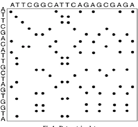
[image:2.595.316.540.375.581.2]The dot-matrix approach, which implicitly produces a family of alignments for individual sequence regions, is qualitative and simple, though time-consuming to analyze on a large scale. It is very easy to visually identify certain sequence features—such as insertions, deletions, repeats, or inverted repeats—from a dot-matrix plot. To construct a dot-matrix plot, the two sequences are written along the top row and leftmost column of a two-dimensional matrix and a dot is placed at any point where the characters in the appropriate columns match—this is a typical recurrence plot. Some implementations vary the size or intensity of the dot depending on the degree of similarity of the two characters, to accommodate conservative substitutions. The dot plots of very closely related sequences will appear as a single line along the matrix's main diagonal.
Fig 1. Dot matrix plot
Dot plots can also be used to assess repetitiveness in a single sequence. A sequence can be plotted against itself and regions that share significant similarities will appear as lines off the main diagonal. This effect can occur when a protein consists of multiple similar structural domains. DNA dot plot of a human zinc finger transcription factor (GenBank ID NM_002383), showing regional self-similarity (Fig 1). The main diagonal represents the sequence's alignment with itself; lines off the main diagonal represent similar or repetitive patterns within the sequence. This is a typical example of a recurrence plot.[7]
3.4
Progressive Method
21 sequences and then adding successively less related sequences
or groups to the alignment until the entire query set has been incorporated into the solution. The initial tree describing the sequence relatedness is based on Pair wise comparisons that may include heuristic Pair wise alignment methods similar to FASTA. Progressive alignment results are dependent on the choice of “most related” sequences and thus can be sensitive to inaccuracies in the initial Pair wise alignments. Most progressive multiple sequence alignment methods additionally weight the sequences in the query set according to their relatedness, which reduces the likelihood of making a poor choice of initial sequences and thus improves alignment accuracy. [7]
4.
METHODOLOGY
The methodology for this work involves the uses the cluster analysis techniques [4][5] to compute the alignment scores between the multiple sequences. Based on the alignment the phylogenetic tree is constructed signifying the relationship between different entered sequences. The data is taken from the databank of NCBI.
4.1
Jukes cantor Method
The Jukes and Cantor model is a model which computes probability of substitution from one state (originally the model was for nucleotides, but this can easily be substituted by codons or amino acids) to another. From this model we can also derive a formula for computing the distance between 2 sequences.
The main idea behind this model is the assumption that probability of changing from one state to a different state is always equal. As well, we assume that the different sites are independent. The evolutionary distance between two species is given by the following formula.
Where Nd is the number of mutations (or different nucleotides) between the two sequences and N is the nucleotide length.[7]
4.2
Algorithm
The algorithm finds the optimal alignment of the most closely related species from the set of species. The work includes the construction of phylogenetic trees for the triticum wheat varies. The sequences for the varieties are loaded from the NCBI database. The phylogenetic distances are calculated based on the jukes cantor method and the trees are constructed based on nearest-neighbor method. The final tree is obtained by using tree pruning. The closely related species are selected based on the threshold condition. As the sequences are very lengthy and the alignment is tedious work for these sequences. To obtain the multiple sequence alignment, the consensus sequence (fixed sequence for eukaryotes) is aligned with the available sequence. This helps in locating the positions near to the optimal alignment. The sequences are aligned based on local alignment and shift right and shift left operations are performed five times to obtain the optimal multiple sequence alignment. The algorithm steps are written below:
Load the m wheat sequences from NCBI database Calculate the distances from jukes cantor method. Create the matrix1 for different species based on JC
distance.
Inspect the original matrix and find the smallest distance. Half that number is the branch length to each of those two taxa (species) from the first Node. Create a new, reduced matrix with entries for the
new Node and the "unpicked" taxa. The distance from each of the unpicked will be the average of the distance from the unpicked to each of the two taxa in Node 1.
Inspect the reduced matrix and find the smallest distance. If these are two "unpicked taxa, then they will form a new Node with branch lengths half that distance. If Node 2 consists of Node 1 plus an "unpicked" taxon, then the branch length to the unpicked will be half the distance and the other branch (with a Node in it) will have two segments adding up to one-half the smallest distance in the matrix.
Continue these distances calculation and matrix reduction steps until all taxa have been picked.
Construct the tree 1.
Load the n more wheat sequences from NCBI database.
Calculate the distances from jukes cantor method. Create the matrix2 for different species based on JC
distance.
Repeat step iv to vi Construct tree 2.
Apply tree pruning to join the tree1 and tree2. Consider the p species above threshold value 0.7. Consider the consensus sequence (TATA box) for
wheat varieties.
Load the p sequences (S1, S2, ……..Sp)
Align TATA consensus sequence with S1 to Sp considering local alignment.
Align the sequences using local alignment with TATA consensus sequence.
Calculate the alignment with shift five shift right and five shift left operations.
Consider the alignment with minimum score.5.
RESULTS AND DISCUSSIONS
22 The Jukes Cantor values for these varieties are shown below.
Columns 1 through 15
2.2840 2.8338 34.2415 2.2956 2.2840 2.3334
3.5762 4.5120 34.2415 1.3255 2.2956 0.7981 1.0927 0.0183 0
Columns 16 through 30
0.0412 0.9284 0.9966 1.7686 1.0740 0.0161 1.0029 0.7850 0.7981 0.7830 0.5973 0.8810 1.3949 1.3432 0.7890
Columns 31 through 45
1.0842 1.0927 1.0590 0.8596 0.6849 0.8790 2.2364 1.0842 0.0183 0.0522 0.9209 0.9863 1.7589 1.0836 0.0021
Columns 46 through 60
0.0412 0.9284 0.9966 1.7686 1.0740 0.0161 0.9092 0.9751 1.7275 1.0985 0.0500 0.8219 1.1671 1.6803 0.9227
Columns 61 through 66
0.9772 1.9545 0.9863 3.3140 1.7589 1.0844
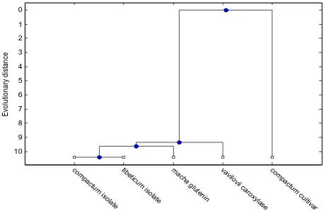
The threshold condition is applied to obtain the most closely related varieties from the set of twelve varieties. The most commonly related varieties are shown in Fig. 4. These varieties are:
'yunnanense_isolate‟ 'vavilovii_isolate‟ 'compactum_isolate‟ 'macha_isolate‟ 'tibeticum_isolate‟
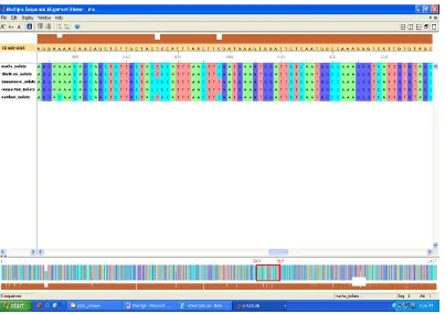
The multiple sequence alignment for these varieties is obtained. The MSA is shown in Fig. 5.
6.
CONCLUSION AND FUTURE SCOPE
6.1
Conclusion
Several different heuristics have been employed over the years to simplify the complexity of the problem of Multiple Sequence Alignment. The pair-wise progressive dynamic programming restricts the solution to the neighborhood of only two sequences at a time. Using this method, all sequences are compared pair-wise and then each is aligned to its most similar partner or group of partners. Each group of partners is then aligned to finish the complete multiple sequence alignment. This is a quite tedious job and is suited for limited number of sequences and also of small length. Also, it doesn‟t guarantee the optimal alignment. One way to still globally solve the algorithm and yet reduce its complexity is to restrict the search space to only the most conserved „local‟ portions of all the sequences involved.
The model is constructed for aligning the DNA sequences of different wheat varieties. There are different sequence formats available from which plain text format is utilized. The two phylogenetic trees are constructed for different datasets.
The closely related sequences are extracted based on the threshold condition. Then the consensus sequence is used for to obtain the local alignment with each sequence. Based on the local alignment, the sequences are arranged at the corresponding positions detected by the consensus sequence. Shift right and shift left operations are performed on each sequence to obtain the optimal alignment.
TABLE1.
TRITICUM WHEAT VARIETIES
S.
No.
Variety Name
Accession Code
1.
Compactum Cultivar
GU259621
2.
Compactum Isolate
GU048562
3.
Compactum
Glutenin
DQ233207
4.
Macha Floral
AY714342
5.
Macha Isolate
GU048564
6.
Macha Glutenin
GQ870249
7.
Sphaerococcum
EU670731
8.
Tibeticum Isolate
GU048531
9.
Yunnanense Isolate
GU048553
10.
Vavilovii Isolate
GU048554
11.
Vavilovii Caroxylase
DQ419977
12.
Gamma Gladin
AJ389678
TABLE I.
23 0 1 2 3 4 5 6 7 8 9 10 co mp act um iso late tib eticu m iso late ma ch a g luten in va vilo
[image:5.595.68.526.85.390.2]vii ca ro xyl ase co mp act um cu ltiva r
Ev
o
lu
tio
n
a
ry
d
ist
a
n
ce
Fig 2. Phylogenetic tree for five wheat varieties
0 1 2 3 4 5 co mp act um cu ltiva r ma ch a flo
ra l va vilo vi i ca ro xyl ase sp ha ero co ccu m co mp act um glute nin ma ch a g luten in gamma g ladin tib eticu m iso late ma ch a iso
[image:5.595.127.474.429.698.2]late co mp act um iso la te yu nn an ense iso late va vilo vi i iso late Ev o lu ti o n a ry d ist a n ce
Fig 4. Phylogenetic tree for five closely related varieties
Fig 5. M.S.A. for closely related species
6.2
Future Scope
Following improvements regarding the developed model of bioinformatics can be made:
The model can be extended for protein sequence alignment.
[image:6.595.99.502.393.678.2]25
7.
REFERENCES
[1] B.Bergeron, Bioinformatics Computing, Pearson Education, 2003, pp. 110- 160.
[2] Clare, A. Machine learning and data mining for yeast functional genomics Ph.D. thesis, University of Wales, 2003.
[3] Han, J. and Kamber M., Data Mining: Concepts and Techniques, Morga Kaufmann Publishers, 2004, pp. 19-25.
[4] Jiang, D. Tang, C. and Zhang, A., “Cluster Analysis for Gene Expression Data”, IEEE Transactions on knowledge and data engineering, vol. 11, 2004, pp. 1370-1386.
[5] Kai, L. and Li-Juan, C., “Study of Clustering Algorithm Based on Model Data”, International Conference on Machine Learning and Cybernetics, Honkong, 2007, Volume 7, No. 2., 3961-3964
[6] Kantardzic, M., Data Mining: Concepts, Models, Methods, and Algorithms, John Wiley & Sons, 2000, pp. 112-129.
[7] Krane, D. and Raymer, M., Fundamental Concepts of Bioinformatics, Pearson Education Publishers, 2006, pp. 1-98.