Color Image Segmentation using Fuzzy Local Texture Patterns

(1)

Color Image Segmentation using Fuzzy Local Texture

Patterns

E. M. Srinivasan

Department of ECE Government Polytechnic College

Thoothukudi, Tamilnadu, India

K. Ramar

Principal

Einstein College of Engineering Tirunelveli, Tamilnadu, India

A. Suruliandi

Department of CSE M S University Tirunelveli, Tamilnadu, India

ABSTRACT

Texture is one of the fundamental image characteristics useful in computer vision tasks such as object recognition and scene analysis. Texture segmentation is one of the image analysis tasks. The prospect of texture segmentation depends on the choice of the texture description method and the segmentation procedure. In this paper, color-texture descriptors are proposed to represent the texture contents of the color images. In these texture description schemes, small areas of the image are represented by fuzzy based local texture patterns and the entire image is represented by frequency occurrence of such texture patterns. Supervised segmentation of color images is performed using these color-texture descriptors and promising results are obtained.

General Terms

Computer Vision, Texture Analysis.

Keywords

Texture Patterns, Fuzzy Local Texture Patterns, Fuzzy Pattern Spectrum, Texture Segmentation.

1. INTRODUCTION

Almost every surface can be regarded with the help of texture, which is a recognizable and indispensable property of the surface. Texture based image analysis plays a vital role in satellite image processing, medical image processing, and many more areas of computer vision. Texture segmentation is one of the texture analysis tasks, which attempts to partition an image into different homogeneous texture regions. The texture description method plays the most important role for efficient image segmentation. Many texture feature extraction methods suitable for segmentation have been proposed by the researchers for gray-level [1 - 5] and color images [6 - 8].

Segmentation is found to be the most complex task in many image processing applications. Segmentation techniques can be classified into either supervised or unsupervised. In the case of supervised texture segmentation, prior knowledge of textures present in the image is required. For unsupervised method of texture segmentation, details of textures present in an image need not be known in advance.

A region based unsupervised texture segmentation method is proposed by Ojala and Pietikainen [2] in which, coarse segmentation and pixel-wise classification scheme are combined and the distributions of Local Binary Patterns (LBP) and the pattern contrast are used as texture descriptor to measure the similarity of adjacent image regions in an image. Muneeswaran et al [1] proposed a feature extraction technique by combining the discriminating texture features of spatial and spectral distribution of image attributes. In this method,

the texture features are extracted by applying Gaussian and Gabor wavelets on the image and they are combined with the local intensity variations to get a combined feature distribution. Then in the segmentation step, the pixels with homogeneous attributes are clustered by fuzzy C-means clustering method and are labeled. A moment based texture segmentation method is proposed by Tuceryan [4] in which, the lower order moments are computed from the image, then the texture features are computed from the moments, and they are used as the texture descriptors for segmentation. Suruliandi and Ramar [9] proposed a one-dimensional histogram based texture description scheme, in which the local texture patterns are used to describe the local texture and the global texture is described by the occurrence frequency of such local descriptors over the entire image. In our earlier paper [10], a fuzzy based method of texture description scheme is proposed and tested for texture classification and texture segmentation of gray-scale images.

Maenpaa and Pietikainen [11] explored different approaches for color-texture analysis. In this paper, color histograms and color ratio histograms which consider only color features are taken into account for texture analysis. In another way, texture features are taken into account. For this, the Gabor filter and LBP operator are used for texture feature extraction. The combination of color and texture descriptions is also analyzed using channel-wise and opponent color-texture description methods. It is concluded in the paper that the performance of the gray-scale texture description method is better than other methods in case of illumination variations. Three different approaches for color texture classification have been proposed by Arvis et al [12], which are based on the co-occurrence matrix method. The first approach is a multispectral extension, in which the co-occurrence matrices are computed within and between color channels. In the second approach, joint color-texture features are computed. The third approach uses the gray-scale texture features computed on the quantized color image. Among the three proposed approaches, the performance of multispectral method is found to be better.

(2)

.

than

greater

if

9

8 ,

1,2,

to

equal

if

1 than

less

if

0 )

,

(















c i c i c i c i

g

i

g

P

v i i

P

ps

S



{

}







8 1 i i

ps

mLTP

)

(

µ

)

µ(

8 1





i i ps

x

mLTP

i ) (mLTP mLTP

FLTP k k

K k µ * 1



 

With reference to Palm [14], the gray-scale texture feature extraction methods can straightforwardly be used for color-texture feature extraction by combining the results from the individual color channels. This simple technique often gives very good results. Since this method does not include inter-channel interactions, it will be robust against illumination color variations.

In this paper, two color-texture description methods are proposed for the segmentation of color images. For local and global texture representation in both methods, Fuzzy Local Texture Patterns (FLTP) model [10] is used. In the first proposed method, to achieve color-texture representation in a simple way, the color image is transformed into a gray-scale image and the texture contents in it are described by the Fuzzy Patterns Spectrum – Gray-Scale (FPSGS). In the next method, to get more effective results, texture features are derived from three individual RGB color channels and are combined to get Fuzzy Patterns Spectrum – Color Channels (FPSCC) to describe the global texture. For the supervised color-texture segmentation, training samples are extracted from different texture regions present in the image and are labeled. During the segmentation stage, each pixel which acts as a test sample is classified and labeled.

The remaining part of the paper is organized as follows. Section 2 describes the texture description methods. In Section 3, the supervised segmentation procedure is explained. Texture segmentation experiments and results are presented in Section 4. Section 5 concludes the paper.

2. TEXTURE DESCRIPTION

2.1 Fuzzy Local Texture Patterns (FLTP)

FLTP method of texture description [13] is used for the local texture pattern formation. In a 3x3 local image region, let gc

be the value of the central pixel and gi(i=1,2,…,8) be the

values of its neighbor pixels. let the difference between gc and

gi be xi (i =1, 2,…, 8). Let the Pattern Unit P, between gc and

its neighbors gi (i =1,2, …, 8) be defined as

(1)

P is assigned with one of the three distinct values 0, 1, and 9 based on the three fuzzy conditions „less than‟, „equal to‟, and „greater than‟. Let µ0(xi), µ1(xi) and µ9(xi) be the membership

degrees of xi to the P values 0,1 and 9 respectively.

The fuzzy pattern unit, FP between gc and its neighbors

gi (i =1,2, …, 8) is defined as

8) , ... 1,2, i ( for ) /9 ) ( , 1 / ) ( , /0 ) ( ( ) ,

(

µ

0

µ

1

µ

9



 i i i

i

c g x x x

g

FP ₍₂₎

If the local region is homogeneous, then the difference between gc and giwill be equal to zero or almost equal to zero.

For this case, µ1(xi) will be higher, µ0(xi) and µ9(xi) will be

lower. In case of non-homogeneous region, the difference between gc and gi will be more and therefore µ1(xi) will be

decreasing, µ0(xi) or µ9(xi) will be increasing.

The local region can be represented as a Fuzzy Pattern Units Matrix (FPUM), in which the entries are FP values. From the FPUM cell values, the FLTP is calculated. Each cell of the matrix contains three membership values associated with the P values (0, 1 or 9). By using these values, a set of Pattern

Strings (S) is constructed. Each S consists of eight elements and is defined by

(3)

where, psi (i =1,2,…,8) is the element of S.

v i

P

means P value of ithelement having non-zero membership value v. If the matrix contains only one non-zero membership value in each cell, there will be only one S. If there are n elements in the matrix having two non-zero membership values, then the total number of S is 2n. S is formed from P values of all possible combinations of non-zero membership values. We use a new mLTP operator is defined by

(4)

When the membership degree values are equal to one in all the matrix elements, there will be only one S and one mLTP. If there are n elements in the matrix having two non-zero membership values, the total number of S and mLTP is 2n. Further, the membership degree to each mLTP is obtained by multiplying the eight membership degrees of corresponding S.

(5)

So, when the 3×3 local region is considered, the central pixel has associated FLTP which is defined by

(6)

where K is the total number of S.

2.2 Fuzzy Pattern Spectrum (FPS)

In the FLTP method, the global texture of the entire image is described by the frequency occurrence of the Fuzzy Local Texture Patterns present in the image and is termed as Fuzzy Pattern Spectrum (FPS). In this paper, color-texture characterization is done by two different methods. In the first method, the color image in RGB color space is transformed into its corresponding gray-scale image. The texture of given image is represented locally by the texture descriptor FLTP and the FLTP values are collected in a one-dimensional histogram FPSGS. In the second method, FLTP are computed for three color channels individually. The frequency occurrence of FLTP corresponding to the three channels are formed and concatenated to get the global texture descriptor FPSCC.

3. TEXTURE SEGMENTATION

3.1 Texture Similarity

(3)

                                                                                             





 



 



      m s n i i m s n i i m s i n

i sm

i n i i m s n i i m s n i i i f f f f f f f f m s G . 1 . 1 , 1 , 1 , 1 , 1 log log log log 2 ) , ( (7)

where s is a histogram of the first image and m is a histogram of second image, n is the total number of bins in the histogram and fi is the frequency at bin i.

3.2 Supervised Texture Segmentation

In the supervised segmentation method, knowledge of textures present in the image is known in advance. So, the training samples of texture regions are extracted and the global texture descriptions are computed for these sampled regions and labels are assigned to them. During the segmentation stage, each pixel is classified and labeled based on the supervised segmentation algorithm. The algorithms for two texture representations are given below.

3.2.1 Segmentation Algorithm for FPS

GS

 Transform the given color image into gray-level image.

 Randomly select sample sub-images from each texture region in the transformed image. Let nt be the total

number of sub-images.

 Calculate FLTP for each sample sub-image using a moving sliding window of size 3x3. Compute FPSGS for all the sub-images

 Scan the transformed image by a sliding window W with a step of one pixel in the row and one pixel in the column directions, calculate the FLTP and compute the FPSGS for each window under consideration.

 Compute the texture similarity G(i), for i = 1, 2, …, nt

between FPSGS of each window with the FPSGS of all model samples.

 Assign the central pixel of the window considered to class I such that G (I) is minimum among all the G (i), for i = 1, 2, …, nt.

3.2.2 Segmentation Algorithm for FPS

CC

 Randomly select sample sub-images from each distinct texture region in the color image. Let nt be the total

number of sub-images.

 Calculate FLTP for each sample sub-image using a moving sliding window of size 3x3 in three color channels. Compute FPSCC for all the sub-images.

 Scan the color image by a sliding window W, calculate the FLTP for three color channels and compute the FPSCC for each window under consideration.

 Compute the texture similarity G(i), for i = 1, 2, …, nt

between FPSCC of each window with the FPSCC of all model samples.

 To assign label to each pixel, follow the last step of Section 3.2.1.

4. EXPERIMENTS AND RESULTS

4.1 Images used in the Experiments

Four mosaic color images are used in the segmentation experiments. They are shown in the first column of Figure 1.

(a) (e)

(b) (f)

(c) (g)

[image:3.595.317.540.123.594.2]

(d) (h)

Figure 1: Input mosaic images and ground truth images

(a), (b), (c), and (d) Input images, (e), (f), (g), and (h) Ground truth images

(4)

Negatives False of Number P ositives True of Number

P ositives True of Number

 

y Sensitivit

correspond to man-made objects. The ground truth image is shown in Figure 1(f). The mosaic image shown in Figure 1(c) of size 512x512 pixels is composed with five texture images from OUTex texture database [17]. The texture images used are Canvas001 (Top Left), Canvas002 (Center), Canvas003 (Top Right), Canvas004 (Bottom Left), and Canvas005 (Bottom Right). All the texture regions correspond to man-made objects. The ground truth image is shown in Figure 1(g). The mosaic image in Figure 1(d) is created using the images of OUTex database. The images used in this figure are Groats007 (Top), Quartz006 (Left), Flakes009 (Bottom), Carpet005 (Right), and Crushedstone003 (Center). The ground truth image is shown in Figure 1(h).

4.2 Experiment #1 : Segmentation of color

images using FPS

GS

The color mosaic images shown in Figure 1 are transformed to gray-scale images and are used as input images in this experiment. All the images are constructed using five different texture regions. The procedure in Section 3.2.1 is used for segmentation. A set of training samples are extracted from the input image. The training set for the classifier consisted of randomly selected sub-image of size 64x64 per texture region. So, there are 5 training samples in total. FPSGS are computed for all the five samples. For every pixel surrounded by a window of size W, FPSGS are computed. The size of window size should be optimum, to bring out the texture properties to discriminate the different texture regions. If the window size is too small, there may be unwanted noisy regions in the segmented output. A larger window size creates boundary problem. Here, a window size of 31x31 is selected. Newly calculated FPSGS of each pixel surrounded by the window is compared with the FPSGS of all training samples using the G-statistics distance measure. The label of training sample with the smallest distance is assigned to the testing sample. All the pixels in the entire input image are classified and labeled. The resulting image is the segmented image. The segmented images are post processed by running a sliding window of size 33x33, and the centre pixel is assigned with the label of majority pixels within the window. The experimental results are given in Figure 2 for the corresponding input texture mosaic images in Figure 1. In the figure, the first column shows the segmented images and second column contains the post-processed images.

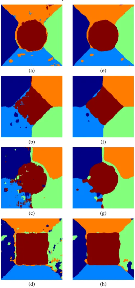
The proposed FPSGS method gives five segments corresponding to the texture regions present in the input images. it is evident from Figure 2(a), FPSGS method suffers in two regions (Sand and Leaves) slightly, because the pattern distributions in these regions are similar in fashion. It is observed from the Figure 2(c) and 2(d), the FPSGS method fails to segment one or two regions correctly. However, in the post-processed images, the noisy patches are suppressed and the results seem to be better.

To evaluate the performance of the proposed method, confusion matrix is used. The confusion matrices for the output images in Figure 2(e)-(h) are given in Tables 1-4 respectively. Diagonal cell entries in the matrix reveal the fact that the number of pixels correctly segmented as mentioned in the ground truth image. This can be referred as True Positives Other cell entries give the number of pixels incorrectly segmented and this is noted as False Negatives. For example, the first row of Table 1 gives the following information. With reference to ground truth image, 43802 Stone texture image pixels are correctly segmented as Stone texture pixels; 74 Stone pixels are misclassified into Sand pixels; 2 Stone pixels

are misclassified into Leaves pixels; 772 Stone pixels are misclassified into Grassland pixels.

(a) (e)

(b) (f)

(c) (g)

[image:4.595.317.540.91.565.2]

(d) (h)

Figure 2: Supervised Segmentation using FPSGS

(a), (b), (c), and (d) Segmented images, (e), (f), (g), and (h) Post-processed images

Sensitivity is one the statistical measures used for the performance evaluation of segmentation algorithms. It measures the proportion of correctly segmented portions to the ground truth. It is defined as

(8)

(5)

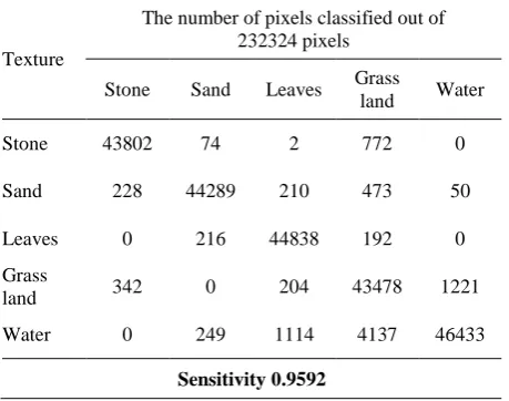
Therefore, the sensitivity for the image shown in Figure 2(e) is calculated from the confusion matrix in Table 1.

Sensitivity =

482 * 482

46433 43478 44838 44289

43802    _{= 0.9592}

Table 1. Confusion matrix for the image in Figure 2(e)

Texture

The number of pixels classified out of 232324 pixels

Stone Sand Leaves Grass

land Water

Stone 43802 74 2 772 0

Sand 228 44289 210 473 50

Leaves 0 216 44838 192 0

Grass

land 342 0 204 43478 1221

Water 0 249 1114 4137 46433

[image:5.595.308.548.86.270.2]

Sensitivity 0.9592

Table 2. Confusion matrix for the image in Figure 2(f)

Texture

Fabric 008

Fabric 007

Fabric 013

Fabric 000

Fabric 015

Fabric

008 44848 171 0 241 101

Fabric

007 750 44602 10 0 0

Fabric

013 0 71 45102 38 151

Fabric

000 0 0 0 45233 128

Fabric

015 196 3239 55 54 47334

[image:5.595.53.283.152.333.2]

Table 3. Confusion matrix for the image in Figure 2(g)

Texture

Canvas 001

Canvas 004

Canvas 005

Canvas 003

Canvas 002

Canvas

001 43966 0 1059 0 89

Canvas

004 1373 39208 986 0 3556

Canvas

005 0 0 44698 310 107

Canvas

003 0 0 1814 43300 0

Canvas

002 1613 680 4286 0 45279

Table 4. Confusion matrix for the image in Figure 2(h)

Texture

Quatz Flakes Carpet Groats Crushed stone

Quatz 37989 530 1207 1457 175

Flakes 0 41729 0 81 0

Carpet 3950 883 34846 1678 453

Groats 1234 0 235 40162 179

Crushed

stone 0 509 430 408 64189

From the Tables, It is observed that the sensitivity is higher for the image in Figure 2(f) and it is interesting to note that better segmentation is visually recognized for the same image.

4.3 Experiment #2: Segmentation of color

images using FPS

CC

Segmentation experiment is carried out as per the procedure explained in Section 3.3.2. Five randomly selected texture sub-images of size 64x64 per texture region are extracted from the input images shown in Figure 1. FPSCC are computed for all the three color channels for five samples of each texture. For every pixel surrounded by a window of size W, FPSCC are computed for each color channel separately. The sliding window size is set to 32x32. The FPSCC of each pixel is compared with the every training sample. The label of training sample with the smallest distance is assigned to the testing sample. All the pixels in the entire input image are classified and labeled. The results are shown in Figure 3. In the figure, the first column shows the segmented images and second column contains the post-processed images.

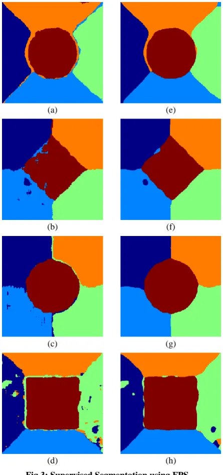
This method is able to achieve better results than the FPSGS method. The segmented images shown in Figure 3(f) and 3(h) contain very few holes. The output images are perceptually very close to the ground truth images shown in second column of Figure 1.

Table 5. Confusion matrix for the image in Figure 3(e)

Texture

Stone Sand Leaves Grass

land Water

Stone 44015 75 2 558 0

Sand 345 44763 139 3 0

Leaves 0 698 44391 157 0

Grass

land 253 132 148 44712 0

Water 11 594 821 4145 46362

[image:5.595.48.287.365.547.2]

(6)

[image:6.595.317.540.70.544.2]

Table 6. Confusion matrix for the image in Figure 3(f)

Texture

Fabric 008

Fabric 007

Fabric 013

Fabric 000

Fabric 015

Fabric

008 45154 9 0 118 80

Fabric

007 1280 44029 53 0 0

Fabric

013 0 24 45195 0 143

Fabric

000 0 0 72 45048 241

Fabric

015 415 2293 64 16 48090

[image:6.595.46.286.90.273.2]

Table 7. Confusion matrix for the image in Figure 3(g)

Texture

Canvas 001

Canvas 004

Canvas 005

Canvas 003

Canvas 002

Canvas

001 45039 0 0 0 75

Canvas

004 606 44421 31 0 65

Canvas

005 87 13 44754 95 166

Canvas

003 110 0 200 44641 163

Canvas

002 508 232 51 166 50901

[image:6.595.46.286.305.486.2]

Table 8. Confusion matrix for the image in Figure 3(h)

Texture

Quatz Flakes Carpet Groats Crushed stone

Quatz 38595 448 2037 27 251

Flakes 0 41781 5 4 20

Carpet 1139 958 38656 748 309

Groats 780 0 317 40546 167

Crushed

stone 5 473 723 62 64273

The confusion matrices for the segmented images in Figure 3(e)-(h) are given in Tables 5-8 respectively. From the tables, it is observed that the sensitivity is more than 0.96 for all the images used in the experiments. The higher sensitivity evidences higher segmentation accuracy.

(a) (e)

(b) (f)

(c) (g)

(d) (h)

Fig 3: Supervised Segmentation using FPSCC

(a), (b), (c), and (d) Segmented images, (e), (f), (g), and (h) Post-processed images

Two benchmark textured images are used in the segmentation experiments. The images of OUTex database are captured under controlled illumination conditions, whereas VisTex images are taken in uncontrolled illumination conditions.

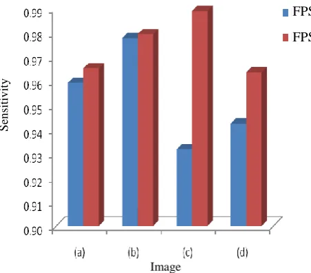
In the first proposed method, the gray-scale texture descriptor is applied on the intensity image which is transformed from the color image. In this method, the color information is not used directly. But, in the second proposed method, texture information in three color channels is represented individually and combined later. So, color and texture features are directly involved in representing images.

[image:6.595.46.287.516.700.2]

(7)

[image:7.595.48.274.125.323.2]

performances of both methods are almost same for the images of VisTex database. But, the performance of FPSCC method is superior to FPSGS method for the OUTex images.

Fig 4: Comparative Analysis of FPSGS and FPSCC models

5. CONCLUSIONS

In this paper, color-texture descriptors are proposed to represent the texture contents of color images. FLTP and FPS are used to describe the local and global texture respectively. The performances of the descriptors have been studied for supervised texture segmentation tasks. One of the approaches for color-texture description is by converting the color image into gray-level image and straightforwardly representing it by the gray-scale texture descriptor. Another approach is describing the texture information of the different color channels individually and combining them later.

From the experimental results of Section 4.2, it is inferred that texture of a color image can be represented by texture descriptor FPSGS that are intended for gray-scale texture. From the results of experiment in Section 4.3, it noted that the second approach of texture descriptor, FPSCC, is performing extremely well for supervised segmentation due to its higher discriminatory power. This much of good performance is achieved at the cost of computing power. From the results, it is noted that the proposed methods give five segments corresponding to the texture regions present in the input images. Therefore, the proposed methods can be used for texture segmentation applications.

In this work, only one-dimensional FPS methods have been focused. Further improvement point of view, segmentation performance may be enhanced by applying co-occurrence features extraction techniques on FLTP and by combining other complementary features like contrast and color. Other popular unsupervised texture segmentation algorithms may be attempted.

REFERENCES

[1] Muneeswaran, K., Ganesan, L., Arumugam, S., and K.,Ruba Soundar, 2006, “Texture image segmentation using combined features from spatial and spectral distribution”, Pattern Recognition Letters, Vol. 27, pp. 755-764.

[2] Ojala, T., and Pietikainen, M., 1999, “Unsupervised texture segmentation using feature distribution”, Pattern Recognition, Vol. 32, pp. 477 – 486.

[3] Raden, T., and Husoy, J.H., 1999, “Texture segmentation using filters with optimized energy separation”, IEEE trans. Image Processing, Vol. 8, pp. 571-582.

[4] Tuceryan, M., 1994, “Moment based texture segmentation”, Pattern Recognition Letters, Vol. 15, pp. 659-668.

[5] Unser, M., 1995, “Texture classification and segmentation using wavelet frames”, IEEE Trans. Image Processing, Vol. 4, pp. 1549-1560.

[6] Chang, M.M., Sezan, M.I., and Tekalp, A.M., 1994, “Adaptive Bayesian segmentation of color images”, Journal of Electronic Imaging, vol. 3, pp. 404-414.

[7] Deng, Y., and Manjunath, B.S., 2001, “Unsupervised segmentation of color texture regions in images and video”, IEEE Trans. Pattern Analysis and Machine Intlligence, vol. 23, pp. 800-810.

[8] Pappas, T.N., 1992, “An adaptive clustering algorithm for image segmentation”, IEEE trans. Signal Processing, vol. Vol. 40, pp. 901-914.

[9] Suruliandi. A., and Ramar, K., 2008, “Local Texture Patterns- A univariate texture model for classification of images”, Proceedings of the IEEE 16th

International Conference on Advanced Computing and Communications (ADCOM08), pp. 32-39. Available online at IEEE Xplore.

[10] Srinivasan, E.M., Suruliandi, A., and Ramar, K., 2011, “Texture Analysis using Local Texture Patterns:A Fuzzy Logic Approach”, International Journal of Pattern Recognition and Artificial Intelligence, Vol. 25, No. 5, pp. 741-751.

[11] Maenpaa, T., and Pietikainen, M., 2004, “Classification with color and texture: Jointly or separately?”, Pattern Recognition, Vol. 37, pp. 1629-1640.

[12] Arvis, V., Debain, C., Berducat, M., and Benassi, A., 2004, “Generalization of the cooccurrence matrix for color images: Application to color texture classification”, Image Anal Sterol, Vol. 23, pp. 63-72.

[13] Drimbarean, A., and Whelan, P., 2001, “Experiments in color texture analysis”, Pattern Recognition Letters, Vol. 22, pp. 1161-1167.

[14] Palm, C., 2007, “Color Texture Classification by integrative co-occurrence matrices”, Pattern Recognition, Vol. 37, pp. 965-976.

[15] Sokal, R.R., and Rohlf, F.J., 1987, “Introduction to Biostatistics”, 2nd

Edition, W.H.Freeman.

[16] VisTex: Texture Database - http://www.vismod.media. mit.edu/vismod/imagery/ visiontexture/vistex.html.

[17] Ojala, T., Mäenpää, T., Pietikäinen, M., Viertola, J., Kyllönen, J. and Huovinen, S., 2002, “OUTex – A new framework for empirical evaluation of texture analysis algorithms”, Proceedings of the 16th International Conference on Pattern Recognition. Image

S

en

siti

v

ity

FPSCC

(8)

AUTHORS PROFILE

E. M. Srinivasan received his B.E. (Electronics and Communication Engineering) in the year 1988 from National Engineering College - Kovilpatti, Madurai Kamaraj University, Tamilnadu, India, and M.E. (Computer Science and Engineering) in the year 1998 from Government College of Engineering - Tirunelveli, Manomaniam Sundaranar University, Tamilnadu, India. He is having more than 23 years of teaching experience. At present, he is working as Upgraded Head of Department, Electronics and Communication Engineering, Government Polytechnic College, Thoothukudi, Tamilnadu, India. He is currently doing Ph.D. in Anna University of Technology, Chennai, Tamilnadu, India. His research interests include Pattern Recognition, Image Processing and Texture Analysis.

K. Ramar received his B.E. (Electronics and Communication Engineering) in the year 1986 from Government College of Engineering - Tirunelveli, Madurai Kamaraj University, Tamilnadu, India, M.E. (Computer Science and Engineering) in the year 1991 from PSG College of Technology, Bharathiyar University, Coimbatore Tamilnadu, India, and Ph.D in the year 2001 from Manomaniam Sundaranar

University, Tamilnadu, India. He has more than 25 years of teaching experience. Currently he is working as Principal, Einstein College of Engineering, Tirunelveli, Tamilnadu, India. He published many papers in International journals and conferences. He organized many National and International conferences. His research interests include Pattern Recognition, Image Processing, Computer Networks and Fuzzy Logic based Systems.