A Robust Biometric Image Texture Descripting Approach

A Robust Biometric Image Texture Descripting

Approach

J Bhattacharya

Central Mechanical Engineering Research Institute Durgapur

West Bengal , India

G Sanyal

National Institute of Technology Durgapur

West Bengal , India

S Majumder

ABSTRACT

The huge demand in online transactions calls for a secure, safe and accurate authentication system .The biometric system such as face, iris, fingerprint, gait has already replaced the existing manual inspection process and surveillance systems in many disciplines. Amongst all these biometrics, face is more attractive as it provides information such as identity, expression, gender, ethnicity and age of an individual.Specially for surveillance purposes,the data acqui-sition for face is much more simpler and can be obtained without the subjects knowledge and cooperation (simply by installing cam-era in public areas) when compared to fingerprints and iris data accumulation.In this paper an edge texture feature using different weight mask coding is utilized for face recognition.Five different sign and difference operators named LSH LC, LSH GC,LDH LC, LDH GC and LSH LGV are developed and used to code the image texture feature.Each image is decomposed into four subset images which are used to generate the texture features. A decision fusion technique is then used for feature classification. The main advan-tage of this approach lies in the fact that they are computationally inexpensive when compared to most texture descriptors.The feature descriptor is applied for face biometric recognition to demonstrate the effectiveness of each approach in extracting textural features.It can also be tested with medical images or other pattern recognition applications.The dataset used for training and testing have consid-erable variances in lighting,viewpoint and other factors so that the potential of the feature extractor, when subjected to any kind of variations, can be judged.

Keywords:

Texture analysis, LBP, Classification, Feature extraction, Face recognitionifx

1. INTRODUCTION

Feature extraction and classification problem is one of the main task undertaken by the computer vision re-searchers.Development of high quality image acquisition sys-tems for perceiving maximum amount of environmental details electronically were carried out in tandem with the advance-ment of information extraction and interpretation techniques.In short,the exact simulation of the task carried out by the vi-sual,neural and cognitive systems of the human body is applied while designing its automatized replica.Any problem statement is thus reduced to a feature extraction and classification prob-lem differing only on the types of features chosen and clas-sification classes from case to case.Features in the visual do-main can be defined as geometric primitives such as point, line, arc segments or some form of derived entities such as color and texture for example.Although a lot of work has been car-ried out on interest point detectors,shape descriptors,edge and line detectors,yet blobs or region patch detection always re-mained an area of focus.This was mainly due to the fact that

these features often require a secondary level of corroboration such as color and texture to make it invariant.This issue is ap-plicable even for human beings where any object is identified more by its color and texture rather than its shape.It is obvi-ous that tasks like pattern recognition,vision based detection of diseased crop,cancer cell detection in medical imaging and many more rely more on textural features.Even in the field of face recognition, techniques based on Geometric matching [1] and Template matching [2] used in the beginning eventually gave way to texture feature extractors for better accuracy and recognition rates.Also, learning models like Support Vector Ma-chines,Neural Network,Hidden Markov Model,which directly used pixel intensity as input components initially [3],[4],started relying on texture features [5].The same applies for techniques like Principal Component Analysis (PCA) , Linear Discrimi-nant Analysis (LDA) ,Independent Component Analysis (ICA), though initially applied over pixel intensities [6] ,[7],[8] have ex-tended to other features [9],[10].Gray-Level Co-occurrence Ma-trices (GLCM’s), Law’s texture measures ,autocorrelation ,prim-itive length, edge frequency , wavelets such as Haar, Morlet, Daubechis and steerable pyramids (GLCM’s) are some com-monly used texture modeling techniques [13, 14, 15, 16].Some notable texture feature extractors specifically designed and ap-plied to face recognition tasks are Wavelets [18],Energy-Entropy features [19],Gabor filters [20] and Local Binary Pattern(LBP) [22, 23].Among these the latter two are mostly used at present . The Gabor filter has the capability of extracting large amount of discriminating local features due to its ability to operate in selec-tive scales and orientations thus capturing the spacial locality and quadrature phase relationships.Usually the gabor kernelψγ,υis

constructed using five scalesυ = 0,1,2,3,4and eight orien-tationsγ = 0,1, ..7hence resulting in a very high dimensional representation thus taking a huge time for computation.

ψγ,υ(z) =kκγ,υk

2

δ2 e

−kκγ,υk2kzk2

2δ2 _[eıκγ,υz_−e−δ2 2_{] (1)}

where κγ,υ = κυeıφγ, δ = 2π, κυ = κmax_fυ , f =

√ 2,

κmax = π₂ ,φγ = πγ₈ ,z = (r, c)andk kdenotes the norm

operation.It can be seen from table 1 that calculating gabor fea-tures for a set of300images takes almost500seconds which is nearly10times that of LBP features.Hence,in many cases the LBP operator is preferred as it is seen that the performance of both are nearly equal.The LBP may also give better result in some cases.For example , the dataset used for experimentation in the proposed work (300 images from the PIE database [24]) gives the highest performance for the LBP operator as shown in table 1.The PIE database created by CMU originally consists of41,368images of68people,considering13different poses,

43different illumination conditions and4different expressions for each person.The300images used for experimental analysis in the present work are selected such that there are images of

op-erator by using the difference magnitude as well as considering the local and global differencing.These texture extractors when applied on a face database shows that some of the techniques perform better than the common LBP operator.The next step lies in feeding the extracted feature information to the classifiers for desired interpretation. A large number of approaches ranging from euclidean or mahalanobis distance classifier to soft comput-ing,linear programming or statistical tools like neural network , Hidden Markov model (HMM) [25], Support Vector Machine (SVM)[11] ,adaboost classifier,bayesian classifier [26],[27] have been developed by different researchers to solve the classifica-tion problem.The present method uses a modified mahalanobis distance classifier to classify the faces.

The contribution of this work can be divided into two parts.Firstly it introduces a new texture descriptor which can be used for different types of object detection and recognition appli-cations.Secondly the decision fusion framework described here can be used for combining any other features for a better recogni-tion rate.The paper is organized in the following manner. Secrecogni-tion 2 provides details about the different developed edge texture op-erators. Section 3 deals with the image classification step.Section 4 shows the results obtained using PIE face database. Finally, conclusion is presented in section 5.

Table 1. Recognition results and Computation time for different features using the PIE Face Database.

Methods Test (in %) Computation time(sec)

LBP 82.6 52

Gabor features 76 500 Daubechies 4 wavelet 74 22.34

Edge Frequency 51.33 58 Laws texture measure 54 41

The results are obtained using LBP,Gabor,Wavelet,Edge Frequency [16],Laws Texture [16] as features and euclidean distance as classifier.

2. EDGE TEXTURE OPERATORS

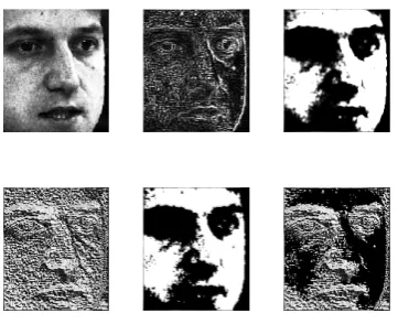
It is a familiar fact that image edges correspond to regions which encompass the substantial information of the scene such as depth & surface orientation alterations and texture & lighting varia-tions.Thus it is obvious that features obtained from these regions provide maximum cue.The operators discussed in this work are hence applied on edge images.Each image is decomposed into the low pas filtered image and the horizontal,vertical and diag-onal edge image.The edge featuresImedge comp

n are obtained

using a kirsch operator over the original imageIm.Generally a kirsch operator gives the edge coefficients in eight directions using8consecutive45degree rotations of the kernel k1 thus yieldingkn, n= 1 : 8.Here the horizontalfh(τ),verticalfv(τ)

and diagonal edge fd(τ) elements are calculated by combin-ing the 2 horizontal(Imedge comp₁ , Imedge comp₅ ) and 2 verti-cal components(Imedge comp₃ , Imedge comp₇ )and the four diag-onal components(Imedge comp2,4,6,8 ). The low pass filtered image

flpf(τ)is computed by subtracting the composite edge image Imedgefrom the original image,where the composite edge

im-age is obtained using the maximum gradient value among all di-rections.The computation steps and results of applying them on an image are further given in equation 9 and figure 1 respectively.

Fig. 1. The lowpass filtered image along with the

horizontal,vertical and diagonal edge components.

k1= 



5 5 5

−3 0 −3 −3 −3 −3



 (2)

Imedge comp

n =Im⊗kn (3)

Im(z)edge= max n=1:8Im(z)

edge comp

n (4)

flpf(τ) =Im−Imedge (5)

fh(τ) = X n=1,5

Imedge comp

n (6)

fv(τ) = X n=3,7

Imedge comp

n (7)

fd(τ) = X n=2,4,6,8

Imedge compn (8)

f(τ) = [flpf(τ) fh(τ) fv(τ) fd(τ)] (9)

The edge texture feature referred asxj,iis then extracted from

each subset image off(τ) individually . Herei ∈ { lowpass image(lp),horizontal edge components(h), vertical edge com-ponents(v), diagonal edge components(d)}. The size ofj de-pends on the number of images used.The feature set for thejth

image can thus be written as{xj,lp,xj,h,xj,v,xj,d}. The

differ-ent operators are further described in the subsequdiffer-ent subsections.

2.1 Local Sign Histogram with Local Center: LSH LC

The sign code of a given pixelfc is computed by finding its

local difference with its neighborsfpand generating the weight

codecs as shown in equation 10.Figure 2 shows the sign and

difference value calculation for a particular pixel.

cs=

7 X

p=0

$p.sp

wheresp=

(

1 (fp−fc)>0 0 (fp−fc)<0

(10)

Four types of weight code $ namely power weight code,gaussian weight code,unity weight code and ordered weight code are used here.These are further elaborated in section 2.6.For obtaining a finer local detail the image is divided into blocks as shown in figure 3 and the frequency magnitude

Fig. 2. (a) A3×3sample window. (b) local difference using the central pixel. (c) sign components for the window. (d) absolute difference components for the

window.

Fig. 3. Face partitioned in equal sized blocks and code

vector is obtained by concatenating the code of all the blocks.

of the number of occurrences f of a particular code with the code value cs as shown in equation 11 .The frequency

referred here is basically the histogram bin value where each bin corresponds to a particular code.

f m(cs) =f(cs)×cs (11)

xj,i= [fm1 fm2 ... fmb] (12)

wherefmn is the frequency magnitude vector of a particular

blockn.This operator is used with the power,gaussian and or-dered weight codes.

2.2 Local Sign Histogram with Global Center: LSH GC

In this operator the sign components are computed for each

3×3window of a block using the global meangcof the

im-age.Equation 10 is hence modified as equation 13.Similar to the LSH LC operator, the LSH GC operator is also used along with the power,gaussian and ordered weight codes.A5×5window can also be used in the same way.Specially for a gaussian weight code,5×5windows are preferred over3×3window as a gentle slope accumulates greater variations thus giving a better result.

cs=

7 X

p=0

$p.sp

wheresp=

(

1 (fp−gc)>0 0 (fp−gc)<0

(13)

The feature setxj,iis calculated in the same way as mentioned

in equation 12.

2.3 Local Difference Histogram with Local Center: LDH LC

Generally only the sign component is used for the LBP operator while the difference magnitude is discarded.[28] used the dif-ference magnitude along with the sign component by coding it like the latter as shown in equation 14.The LDH LC operator is tested with a different coding technique where the frequency is updated after calculating the difference components(as shown in figure 2d) for each3×3window of a block as shown in equation 15.

cm=

7 X

p=0

2p.mp

wheremp=

(

1 kfp−fck −gc>0 0 kfp−fck −gc<0

(14)

H(dp) =H(dp) + 1,∀p= 0, ....,7

wheredp=kfp−fck (15)

H(dp)gives the histogram ofdp.As the value ofdpranges from 0−255,its frequency is generated directly without using any weight code.For generalization it is considered that it uses the unity weight code(which implies no weight multiplication and no summation).

xj,i= [H(dp)1 H(dp)2 ... H(dp)b] (16)

2.4 Local Difference Histogram with Global Center: LDH GC

In this operator the difference components are computed for each3×3 window of a block using the global meangc of

the image.The frequency is then updated as shown in equation 17.Using the global mean while calculating the difference com-ponents is much less error prone than the local center case as the latter is highly sensitive to noise.

H(dp) =H(dp) + 1,∀p= 0, ....,7

wheredp=kfp−gck (17)

As in LDH LC,LDH GC also uses the unity weight code. The feature setxj,iis calculated in the same way as mentioned in

equation 16.

2.5 Local Sign Histogram with Local & Global Variation: LSH LGV

Noise sensitivity can further be reduced if relative differences are considered.In LSH LGV two difference components are cal-culated as shown in equation 18.First the local differencedpis

calculated and then the differencembetween the local centerfc

and the global meangcis calculated.The sign code is then

calcu-lated using the difference between these two values as shown in equation 19.

dp=kfp−fck

m=kgc−fck (18)

cs=

7 X

p=0

$p.d

whered=

(

1 dp> m 0 dp< m

(19)

This operator is used with the power,gaussian and ordered weight codes. The feature setxj,iis calculated in the same way as

amount of information depicted by the sign and difference com-ponents using local and global center differencing and the sign components using local and global variations.

Fig. 4. The top row shows the original image , difference

components using local & global differencing from left to right. The bottom row depicts the sign components using local & global

differencing and local global variation from left to right.

2.6 Weight Codes

As mentioned previously four different types of weight codes are used as shown in figure 5.In case of a power weight mask,the mask coefficients are generated using the power of real numbers

ras$=rp_{,wherep= 0,1, ..7.The binary(r= 2)code}

com-monly used in LBP is an example of the power weight code. For ordered weight codes the pixel position1−8can be weighted using natural numbers1−8,even numbers 2−16,odd num-bers1−15,fibonacci series 1,1,2,3, ..,21or prime numbers

1,2,3, ..17while the gaussian weight codes uses a gaussian ker-nel as weights.The size of the feature vector also depends on the type of code used.For example,for a power code ofr = 1.5the feature size of each block is50.This size is actually obtained from the summation of the kernel (shown in figure 5) used.Thus the total size for an image divided into16blocks gives a size of

800for each feature(lp, h, v, d). The performance variation on the basis of ther valuefor power kernels,s valuefor gaussian masks andtype of numberingfor ordered weights are later dis-cussed in section 4.Five variations are disdis-cussed for each type as shown in table 2.

Fig. 5. Examples of some weight code kernels for gaussian

(standard deviation s=1.5 and 2.5),power weights (r=1.5 and 2.5) and ordered weights.

Table 2. Variations of each type of weight code.

Power Weight (r) Gaussian Weight (s) Ordered Weight 1 1.5 1.5 Odd numbers (1:15) 2 1.75 1.75 Even numbers(2:16) 3 2 2 Natural numbers (1:8) 4 2.25 2.25 Prime numbers (1:17) 5 2.5 2.5 Fibonacci (1:21)

3. IMAGE CLASSIFICATION

The feature descriptorxis further transformed in the eigen space using equations 21 to 24.

x=



  

x1,lp x1,h x1,v x1,d

x2,lp x2,h x2,v x2,d

..

. ... ... ... xm,lp xm,h xm,v xm,d



  

(20)

Here, each element is referred asxj,ii.e. theithfeature set of the jth_{image .An entire rowx}

j,:represents all the features of thejth image{xj,lp,xj,h,xj,v,xj,d}whereas an entire columnx:,i

de-notes theith_{feature of all themimages.Each featurex}

:,i here

is transformed to the eigen space individually and their dissimi-larityσiis computed.These are then fused as shown in equation 26to determine the fused dissimilaritysigmacomb. The mean

vector of each featureiis calculated using equation 21.

µi= m

X

j=1

xj,i (21)

The covarianceCiof the featureiin the training set is calculated

as shown in equation 22

Ci= 1 mϕ

T

i ×ϕi (22)

whereϕiis the mean adjusted data for featurei.The feature is

then transformed to the eigen space using the eigen vectorsωi

of the covariance matrixCi as shown in equation 23.It should

be noted that the subscriptihere on is used to refer a particular feature set generated using all the images.Hence the following computations is to be carried out for all the four features before determining the combined dissimilarity vector.

Ωi=ωT i.ϕ

T

i (23)

For any test image the transformed vector in the eigen space is calculated from the featureˆxk,iusing equation 24.

b

Ωk,i=ωTi.(ϕbk,i)

T

(24)

where

b

ϕk,i= ˆxk,i−µi (25)

The dissimilarity vector σi (σi = {σ1,i, σ2,i, ..., σm,i}) is

calculated by finding the mahalanobis distance between each training image projection component vectorΩj,iand test image projection component vectorΩk,ib . The combined dissimilarity

σcombis then obtained using equation 26 and the best match is

given by the image producing the least dissimilarity.

σcomb= (

X 1

σi

)−1 ₍₂₆₎

It can be proved that using this multimodal combination ,the dissimilarityσcomb obtained by combining all the variables is

less than the individual dissimilarityσifor eachi. This can be

1 2 3 4 5 265

270 275 280 285 290 295 300

num of recognized images

ordered power gaussian

Fig. 6. The graph represents the performance of the weight codes

with the different parameter types.The parameter selection is carried out using the LSH GC operator over the lowpass filtered

image.

σcomb> σ1. Thus

1

1

σ1+

1

σ2 +· · ·+

1

σn

> σ1

⇔ 1

σ1

> 1 σ1

+ 1 σ2

+· · ·+ 1 σn

The above identity is wrong for all values ofσ1asσ1is a square root of a squared term and hence is always positive.Thus the above assumption is wrong and it can be stated thatσcomb < σ1. σcomb is similarly less than σ2, σ3... Hence it is seen that σcomb is less than the dissimilarities of all the variables

and also decreases with the increase in the number of vari-ables.The basic aim of using a multiple feature set is to reduce the false alarms or wrong identification obtained while depend-ing on a sdepend-ingle feature.A multi dimensional feature set can ex-tract more salient information thus solving the problems of view-point,scale,illumination and other changes of the scene to some extent.However, feature fusion often hampers the overall perfor-mance in cases of samples which gives a good detection rate for one feature but a poor one for another.The above approach serves the advantage of using a multimodal feature set safely avoiding the general drawback as explained above.

4. EXPERIMENTAL RESULTS AND DISCUSSION

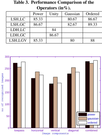
The performance analysis of the operators is carried out using the PIE face database with a set of300images (15different individu-als with20images each).For all the cases10out of the20images were used for training.The face images were normalized to a di-mension of 150 x 130 pixels before use.The performance varia-tion among the five types of parameters for each weight code (as discussed in table 2) is provided in figure 6.The LSH GC oper-ator is used for the results shown in tables 4 and 5 and figures 6 and 7. It is seen that for the power weights and gaussian weights the performance decreases when thervalueor standard devia-tion (as applicable) is increased.The optimal performance is at-tained atr= 1.5ands= 1.5for the power and gaussian weight codes respectively while the the odd and even ordered weight codes give a more or less similar performance.Using these opti-mal parameters for each weight code the different operators are evaluated as shown in table 3. It is observed that all the operators gives a more or less similar performance,however the LSH GC gives the maximum recognition rate for the current dataset.From table 3 and figure 6 it can be inferred that the performance of

Table 3. Performance Comparison of the Operators (in%).

Power Unity Gaussian Ordered LSH LC 85.33 80.67 86.67 LSH GC 86.67 82.67 89.33

LDH LC 84

LDH GC 86.67

LSH LGV 85.33 80 88

lowpass horizontal vertical diagonal combined 0

50 100 150 200 250 300

Image components

no of recognized images

power gaussian ordered

Fig. 7. The graph depicts that the three edge components give a

higher recognition rate with gaussian weights than the ordered or power weights.

the gaussian weights is slightly lower than the power and or-dered weights.Figure 7 further shows the recognition rate for each weight code obtained using the individual image compo-nents as well as the combined rate.A few conclusions are ob-tained from this result.Initially,it is noticed that the recognition rate from the lowpass image is less for the gaussian weight code when compared to the other two,hence resulting in the over-all performance decrease.However the performance of the other edge components are slightly better than those obtained from the power and ordered weight codes.Thus combining a power/order coded lowpass image with gaussian coded edge components may result in an effective performance hike (seen in table 4).It can also be confirmed that the multimodal distance metrics gives a satisfactory result as it is not influenced by the low performance of particular features (for example the vertical component gives a low recognition for all the weight codes,yet its removal low-ers the combined performance by1.8%approximately) and in-creases the overall performance considerably (as distinctly no-ticed in case of gaussian weight code).

Table 4. Performance Comparison of Different Weight Combinations (in%).

G1.5σ G1.75σ G2σ

Ordered natural no. 92.67 92.67 90.67 Ordered odd no. 93.33 92.67 90.67 Ordered even no. 92.67 92.67 90.67 Ordered prime no. 93.33 92.67 90.67 Ordered fibonacci no. 92 91.33 90

Power r=1.5 92.67 90 90

power and ordered codes work better with the frequency mag-nitude descriptor.Also,there is no improvement while combining the different components of the power and ordered codes.

Table 5. Performance Comparison with modified gaussian (in%).

G1.5σ G1.75σ G2σ

Frequency magnitude 81.33 80 77.33 Frequency 89.33 89.33 88.67 Freq mag with Ordered natural no 92.67 92.67 90.67 Freq with Ordered natural no. 95.33 93.33 92.67

5. CONCLUSION

The experimental results verify that all the operators give a fairly high performance in classifying the images reliably with negli-gible false alarm or wrong identification with a high accuracy and low processing time.The feature set calculation time for300

images is approximately90sec which is much less when com-pared to the statistical textural descriptors .The LSH GC oper-ator gives the best performance for the current dataset.It is also seen that the gaussian weights perform better on the edge com-ponents while the power/ordered weights give a better recog-nition rate for the lowpass filtered image.Combining the gaus-sian and power/ordered weights give a fairly high recognition rate(95.33)when compared to the LBP operator which gives a recognition rate of82.6for grayscale intensity images and84.67

when used on edge images used for the present work.On a de-tailed observation,it was found that the main difference in these performances occur in cases of expression variations,especially eye region.The present technique is more expression invariant than the traditional LBP technique.The present code is tested on an Intel Pentium 4 machine, with CPU 3GHz and Memory 1GB using Matlab 7.0.As the face database used for testing has huge variations in pose,expression,orientations and lighting con-ditions;it can be inferred that the proposed technique is resilient to these variations and can give a robust performance in any kind of environment.The technique can be applied to different kind of detection and recognition tasks ranging from pattern recogni-tion like face or gesture to medical imaging applicarecogni-tions. Work is in progress to apply the feature extractor for medical imaging operations.

6. REFERENCES

[1] S. Tamura, H. Kawa, and H. Mitsumoto, “Male/Female identification from 8x6 very low resolution face images by neural network,”Pattern Recognition, vol. 29, pp. 331-335, 1996.

[2] R. Bruneli and T. Poggio, “Face recognition: features ver-sus templates,” IEEE Transactions Pattern Analysis and Machine Intelligence, vol. 15, pp. 1042-1052, 1993. [3] N. Jamil, S. Iqbal, N. Iqbal, “Face Recognition Using

Neu-ral Networks,” IEEE Proc. of INMIC technology for the 21st century, pp. 277-281, 2001.

[4] P. J. Phillips, “Support vector machines applied to face recognition,”Advances in Neural Information Processing Systems 11, MIT Press, 1999.

[5] Bhaskar Gupta , Sushant Gupta , Arun Kumar Tiwari,Face Detection Using Gabor Feature Extraction and Artificial Neural Network

[6] M. Turk and A. Pentland, “Eigenfaces for recognition,”

Journal Cognitive Neuroscience, vol. 3, pp. 71-86, 1991. [7] Martinez, A.M., Kak, A.C., “PCA versus LDA,” IEEE

Transactions Pattern Analysis and Machine Intellgence

Vol. 23 (2), pp. 228-233, 2001.

[8] M. S. Bartlett, J. R. Movellan, and T. J. Sejnowski, Face Recognition by Independent Component Analysis, IEEE Transaction on Neural Networks, Vol 13, pp. 1450-1464, 2002.

[9] Xiaoyang Tan and Bill Triggs,Fusing Gabor and LBP Fea-ture Sets for Kernel-Based Face Recognition,Springer Ver-lag,2007

[10] YUCHUN FANG, ZHAN WANG,IMPROVING

LBP FEATURES FOR GENDER

CLASSIFICA-TION,Proceedings of the 2008 International Conference on Wavelet Analysis and Pattern Recognition, Hong Kong [11] C. J. C. Burges, “A tutorial on support vector machines for

pattern recognition,”Data mining and knowledge discov-ery, Vol.2, pp. 121-167, 1998.

[12] Guoqin Cui, Wen Gao, Feng Jiao, and Shiguang Shan, “Face Recognition Based on Support Vector Method,”

Asian Conference on Computer Vision, January 2002. [13] M. J. Nassiri and A. Vafaei and A. Monadjemi and Pwaset,

” Texture Feature Extraction Using Slant-Hadamard Trans-form”,World Academy Of Science, Engineering And Tech-nology, 2006.

[14] Yuxin Liu and Yanda Li, ” Image Feature Extraction And Segmentation Using Fractal Dimension”,IEEE Conference on Information, Communications and Signal Processing, 1997.

[15] Hua Yuan and Xiao-Ping Zhang and Ling Guan, ” A Statistical Approach For Image Feature Extraction In The Wavelet Domain”,IEEE Conference on Electrical and Computer Engineering, 2003.

[16] Mona Sharma,Markos Markou,Sameer Singh, ” Evaluation of Texture Methods for Image Analysis”,Pattern Recogni-tion Letters.

[17] Cootes, T.F., Edwards, G.J., Taylor, C.J., “Active Appear-ance Models,” Proc. European Conf. on Computer Vision, Vol. 2, pp. 484-498, Springers, 1998.

[18] Yi Liu,Tao Sun , Huang Yang , Yongmi Yang , Xinhong Zhou ,Wavelet-Based Face Recognition Method by Using Support Vector Machine,Innovative Computing, Informa-tion and Control (ICICIC), 2009 Fourth InternaInforma-tional Con-ference, 2009

[19] Cunjian.chen Jiashu.zhang,” Wavelet Energy Entropy as a New Feature Extractor for Face Recognition”, Fourth Inter-national Conference on Image and Graphics,IEEE ,2007. [20] Chengjun Liu, Harry Wechsler, “A Gabor Feature Classifier

for Face Recognition,”Proceedings of ICCV, pp. 270-275, 2001.

[21] T. Ojala, M. Pietikinen, T. Menp, “Multiresolution gray-scale and rotation invariant texture classification with lo-cal binary patterns,”IEEE Transactions on Pattern Analy-sis and Machine Intelligence, vol. 24, pp. 971-987, 2002. [22] T. Ahonen, A. Hadid, and M. Pietikinen, “Face Recognition

with Local Binary Patterns,”Proc. Eighth European Conf. Computer Vision, pp. 469-481, 2004.

[23] T. Ojala, M. Pietikinen, T. Menp, “Multiresolution gray-scale and rotation invariant texture classification with lo-cal binary patterns,”IEEE Transactions on Pattern Analy-sis and Machine Intelligence, vol. 24, pp. 971-987, 2002.

[24] CMU,PIE Face Database,http :

//www.ri.cmu.edu/researchprojectdetail.html

[25] F. Samaria and F. Fallside, “Face identification and feature extraction using hidden markov models,”Image Process-ing: Theory and Application, Elsevier, 1993.

[27] S. Avidan, “Support Vector Tracking,” In IEEE Confer-ence On Computer Vision And Pattern Recognition (Cvpr), 2001.