The use of Bayesian statistics to predict patterns of spatial repeatability

THE USE OF BAYESIAN STATISTICS TO PREDICT

PATTERNS OF SPATIAL REPEATABILITY

Authors: Simon P. Wilson1_{, Niall K. Harris}2_{, Eugene J. OBrien}3

1. Fellow & Senior Lecturer, Department of Statistics, Trinity College Dublin, Ireland.

2. Research Assistant, School of Architecture, Landscape & Civil Engineering, University College Dublin, Ireland.

3. Professor of Civil Engineering, University College Dublin, Ireland.

Abstract:

sensitivity of the model to errors in parameter estimation is discussed, as is the potential for implementation of the method.

Key words: weigh-in-motion, statistical spatial repeatability, Bayesian, pavement, impact factor

Corresponding Author: Niall K. Harris

Email: [email protected]

Tel: +353 1 716 7259

NOMENCLATURE

cb = Vehicle damping coefficient Gd = Pavement spectral density g = Acceleration due to gravity

IF = Impact Factor

IFonm = Observed Impact Factor for truck n at location m K = Mean suspension stiffness of fleet

Kt = Mean tyre stiffness of fleet

k = Suspension stiffness

kn = Suspension stiffness of truck n

kt = Tyre stiffness

ktn = Tyre stiffness of truck n

M = Number of sensors

m1 = Unsprung mass

m2 = Sprung mass

m2n = Sprung mass of truck n

N = Number of vehicles

P = Static vehicle weight

R(t) = Vehicle tyre force

r(t) = Road profile height at time t

t = Time

v = Vehicle velocity

z = Lateral approach position

zn = Lateral approach position of truck n

IF2 = Unknown error in IF

k2 = Variance in suspension stiffness kt2 = Variance in tyre stiffness

1. INTRODUCTION

Spatial repeatability is the phenomenon that the pattern of dynamic force applied by a truck axle to a road pavement is similar in repeated runs at the same speed. This effect results in a concentration of high dynamic tyre forces at specific locations on a pavement surface and has been observed by several authors both experimentally [1,2] and in numerical studies [3]. This opposes the traditional assumption that applied dynamic tyre loads are randomly distributed along a pavement length, suggesting that the pavement is uniformly susceptible to damage along its length.

Cole & Cebon [4] performed a numerical investigation of spatial repeatability using an experimentally validated two-dimensional articulated vehicle model. They generated a fleet of thirty-seven leaf sprung vehicle models with similar geometry and eight varying parameters relating to the ride characteristics, identifying repeatable patterns of dynamic tyre forces. The relationship between vehicle velocity and level of repeatability was highlighted. A further experimental study, involving measurement of heavy vehicle tyre forces on a major national route in the UK, was conducted [5] which confirmed theoretical predictions of the influence of speed on spatial repeatability of tyre forces.

SSR has great implications for pavement deterioration. Pavement deformation and damage is directly related to impact force and the pattern of SSR is related to the road profile. It seems likely therefore that the process of road pavement deterioration is integrally linked with SSR. Following some initial imperfections, road surface deformations are generated which result in a pattern of SSR. The repeatable forces cause further deformation which may reinforce the existing pattern of SSR or change it.

Some research has focused on integrated pavement deterioration models for the calculation of pavement life [7], dividing the procedure into four main areas: dynamic vehicle simulation, pavement primary response calculation, pavement damage calculation and profile change and damage feedback mechanisms. Within this context, it is clear that the accurate prediction of applied dynamic forces is necessary for the calculation of long-term pavement performance.

This paper describes a method to predict the pattern of SSR. A quarter-car model (Figure 2) is used to calculate the force applied to a pavement as it travels at a given speed. The pavement surface is modelled as a three-dimensional ‘carpet’ to provide a varied but correlated series of road profiles for the vehicle model. The profile chosen from the 3-D surface depends on the lateral approach position of the vehicle model.

distributions for the properties, if known, can be used to predict the pattern of SSR. Using Bayesian updating [8], these distributions can be updated through comparisons between calculated and measured impact forces. In this study, the approach is tested using Monte Carlo simulation to generate distributions of impact forces corresponding to a vehicle fleet whose properties have known statistical distributions. With Bayesian Updating, a heavy vehicle fleet model is determined which can be used to predict patterns of SSR.

2. VEHICLE MODEL

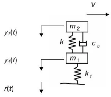
The Bayesian approach is tested using the quarter-car model of Figure 2 which represents an individual heavy vehicle axle. The model, which travels at constant velocity, v, has two degrees-of-freedom, corresponding to body bounce, y2(t), and axle

hop, y1(t), vertical motions. The vehicle is excited by pavement roughness, r(t). This

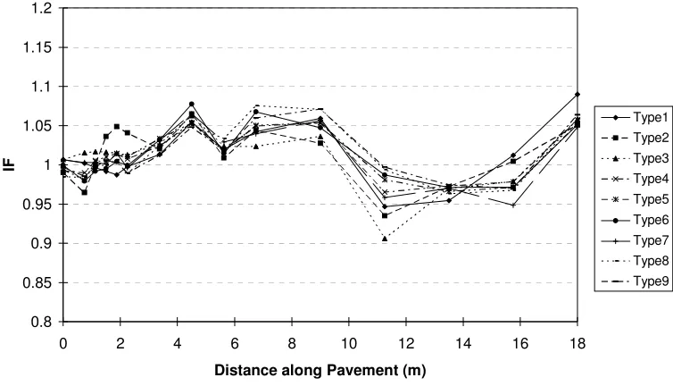
modelling approach clearly neglects certain characteristics of heavy vehicle ride, such as the load sharing effect between heavy vehicle axle groups (tandems, tridems, etc.) as well as vehicle pitching and rocking motions. However, it was judged to be sufficient to detect the basic pattern of SSR which was found by to be substantially independent of the number of axles in the vehicle (see Figure 1) [6].

There are six variables in the quarter-car pavement interaction model:

kt = tyre stiffness

cb = suspension damping z = lateral approach position

The effect of tyre damping is assumed to be negligible, and thus is not considered. The system is further simplified by assuming constant values for vehicle unsprung mass and suspension damping coefficient.

It is implicitly assumed that impact force data will be collected from a multiple-sensor weigh-in-motion system such as that being developed in the WIM-HAND project [9, 10]. Hence, high accuracy estimates of the sprung mass, m2, will be available by

averaging the measurements from the many sensors or using a more elaborate algorithm to process the multiple force measurements [11].

This reduces the number of variables to four, one of which, m2, is known and three, k, kt and z whose distributions are sought. The three unknown variables are assumed to

be Gaussian distributed with unknown mean and variance, and values observed for each truck are also assumed unknown.

The quarter-car model is used to simulate the motion of the fleet of vehicle axles and hence to reproduce the pattern of SSR. The distributions of its three unknown parameters are found by Bayesian updating.

(1)

(2)

where R(t) is the tyre force imparted to the pavement, given by:

(3)

The impact factor, IF, is then given by normalising the dynamic tyre force by the corresponding static vehicle weight:

1 2

( ) ( )

( )

R t IF t

g m m (4)

2.1 Road Profile Generation and Filtering

spectral densities of the profile, Gd(n), are generated using British Standard

classifications for road roughness [12], given by:

(5)

where n is the wavenumber in cycles/m, n0 = 0.1 cycles/m and Gd(n0) and w are

constants related to the surface roughness of the pavement. The spectral density is subjected to a two-dimensional inverse Fourier transform to produce a discrete set of points representing the profile height, r(t), at regular finite longitudinal and lateral intervals [13]. Three profile surfaces are generated for use in this study, the first two (AS1, AS2) having a roughness coefficient of 6

0

( ) 20 10

d

G n m3/cycle,

corresponding to a class ‘B’ road (good quality highway). The third profile (AS3) is a class ‘C’ pavement (national road) with a roughness coefficient of 6

0

( ) 64 10

d

G n

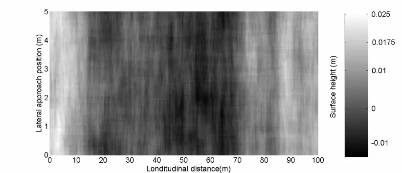
m3/cycle. Each section of road generated measures 100 m in length and 5.0 m in width (Figure 3). The sections of randomly generated road profile are then subjected to a moving average filter to simulate the envelopment of short wavelength disturbances by the tyre contact patch [14]. A base wavelength of 0.3 m is chosen for this purpose.

3. BAYESIAN STATISTICAL INFERENCE

variables of the quarter-car that are most consistent with these data. Such fitting can be attempted through a wide variety of numerical methods, for example, minimizing least squares using gradient descent or other optimization approaches.

For data on several trucks, the procedure could be applied independently to each. However this ignores important information in such data about the overall distribution of variable values across the total population of trucks. Extracting this information then allows hypotheses to be tested and predictions made about the fleet, rather than being restricted to statements about the observed trucks only. This information is in the form of the probability distribution of the values of the quarter car model variables, k, kt and z.

The following notation is adopted. Impact factor from N trucks measured at M

locations on the road surface is acquired, where IFonm is the observed impact factor

from truck n at location m. The quarter car variables for truck n are subscripted: kn, ktn, m2n, zn.

3.1 A Fleet Model for Impact Factors

An allowance is made for the possibility that the observed impact factor for truck n at location m, IFonm may be subject to some error from that given by the quarter car

model. This error is composed of deviations in the real system from the model and measurement error of the sensor. Gaussian distributed error is appropriate in this case with a mean given by the quarter car model. Thus the observed impact factor of truck

n at location m is described by:

2 2

~ N( ( ; , , , ), )

o

nm n m n tn n n IF

IF IF t k k m z (6)

where X ~ N( , 2) means that X is a variable that is Gaussian distributed random variable with mean and variance 2. IFn(tm; kn, ktn, m2n, zn) is the impact factor

according to the model of Section 2 for truck n at location m with given quarter-car parameters kn, ktn, m2n and zn. IF2 is the unknown error at the time at which the truck

impacts on the mth sensor location.

The expected value of the observed impact factor, IFn(tm; kn, ktn, m2n, zn), given by

population distribution. The distributions of these variables are considered to be Gaussian with unknown means and variances:

2

2

2

~ N( ,

)

~ N( ,

)

~ N( ,

)

n k

tn t kt

n z

k

K

k

K

z

Z

for n = 1,...,N.

The unknown variables in the problem are then kn, ktn, zn, n = 1...N, and K, k2, Kt, kt2, Z, z2 and IF2 which will be found. As previously stated in section 2, the remaining

variables of the quarter-car model, unsprung mass, m1, and suspension damping, cb,

are assumed constant for all trucks and known. Sprung mass, m2, which varies between vehicles, is estimated here by taking the mean impact force for each quarter car, and subtracting the constant unsprung mass, m1. Additionally, truck velocity is assumed to be constant and is easily determined from the time interval between simulated sensor measurements. The road surface profile at the site and the immediate approach is assumed measurable and known.

3.2 Bayesian Inference

Applying Bayesian inference, a probability distribution is computed over the unknown variables given the data (the posterior distribution):

2 2 2 2

p( , , , 1, ..., ; , , , , , , | o ; 1, ..., , 1, ..., )

n tn n k t kt z IF nm

where p(x | y) represents the probability distribution of the vector of variables x conditional on observing the vector of values y. By Bayes law, this can be written as (Lee 2004):

2 2 2 2

2

2 2

p( , , , 1, ..., ; , , , , , , | ; 1, ..., , 1, ..., )

p( ; 1,..., , 1,..., | , , , 1, ..., ; )

×p( , , , 1, ..., | , , ,

o

n tn n k t kt z IF nm

o

nm n tn n IF

n tn n k t kt

k k z n N K K Z IF n N m M

IF n N m M k k z n N

k k z n N K K 2

2 2 2 2

, , )

p( , , , , , , )

z

k t kt z IF

Z

K K Z

(9)

The first and second terms on the right hand side of the above expression are the product over n and m of the Gaussian probability functions of Equation 6 and Equation 7. The prior distribution must be defined in addition to the model and describes the state of knowledge of the parameters before the experiment is conducted (i.e., the posterior distribution from similar experiments that have been conducted previously). For this paper it is assumed that no prior knowledge of these parameters exists, which is modelled by assuming the prior to be uniform distributions over a very large range (much larger than the range of values for the parameters that is believed possible).

simulation, such as Monte Carlo integration, allow for the construction of approximations to the posterior distribution or functions of it, such as means [17].

3.3 Predictions and Assessment

Once the posterior distribution is approximated, it is used for two purposes:

1. Construction of the distribution of values of quarter car variables in the fleet. This distribution describes the probability that a randomly selected truck from the fleet has a certain combination of values of the variables used in the quarter-car model.

2. Model checking. Using this distribution, it becomes possible to infer the probability distribution of impact factors that would be observed given this distribution on the quarter-car variables. Usually this is done by simulation; values of the quarter-car parameters are simulated from the distribution and impact factors are then computed through the deterministic model of Section 2. An observed impact factor is then simulated from the Gaussian distribution with the mean impact factor and variance that is simulated from the posterior distribution. The distribution is then compared with the observed data (see section 4). This procedure checks that the fitted model, with all its assumptions, is consistent with observed data.

4. THEORETICAL TESTING

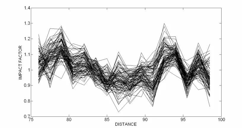
kt, z, v and m2 and constant values for cb and m1. This fleet size was chosen to minimise computation time as well as to test the robustness of the algorithm for a relatively small data set. Using normally distributed velocities and lateral approach positions, the theoretical vehicle fleet is then subjected to the disturbance input from the road profile surface described in section 2.1 and time histories of vehicle tyre force are output. For each vehicle in the fleet, the dynamic tyre forces at sixteen WIM locations, assumed to be equally spaced 1.5 m apart from 76 m to 98.5 m longitudinally on the road surface, are recorded and input to the Bayesian inference algorithm described in section 3, which is initiated using assumed distributions for k,

kt and z. The preceding 76 m of approach pavement is used to allow the vehicle model

to attain dynamic equilibrium. As previously stated, it is assumed that the velocities of each individual vehicle, the local road profile and the GVW of each vehicle may be reasonably determined in practice and as such, are considered known quantities to the Bayesian inference algorithm.

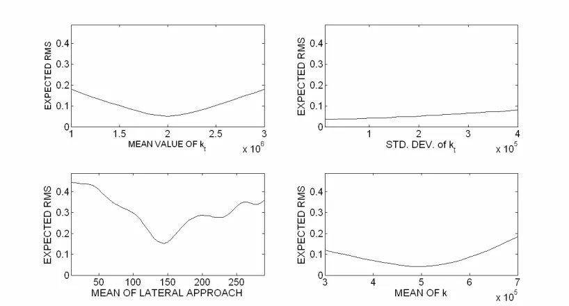
For the Bayesian Updating approach to be successful, it is necessary that the impact factors used are sensitive to the vehicle parameter values. The root mean square (RMS) error in impact factors for some of the input parameters is shown in Figure 5. In each case, all other model parameters are fixed to the nominal values. It can be seen that the standard deviation of kt tends to have little effect on the overall RMS

error, with similar behaviour exhibited for the standard deviations of k and z. The error due to variation in the parameter mean values is greater, particularly so for lateral approach. This is because the mean disturbance input to the vehicle model can vary significantly with lateral position, especially for rougher profiles.

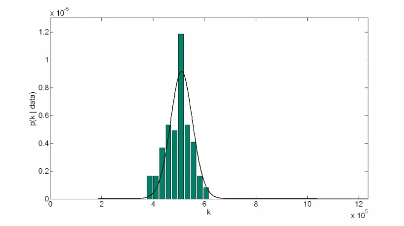
The effectiveness of the Bayesian statistical inference procedure is illustrated in figure 6, which compares the fitted distribution of spring stiffness, k, and the histogram of the observed data. As can be seen, good agreement exists between inferred and true distributions, with similar results obtained for tyre stiffness, kt, and lateral approach

position, z.

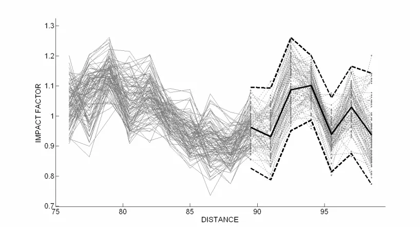
In figure 8, the truck fleet properties are determined from the first 10 points of the WIM array only and the fleet model is tested with the remaining 6 data points. The mean and 95% prediction limits illustrated for the last 6 points are based on a fleet model derived from IF data from the first 10 points. The limits are compared in the figure to data generated using the true properties. It can be seen that the fitted distribution is effective in predicting the range of observed impact factors at each location as well as the pattern of SSR, noting that the fitted model predicts correctly that sensors 12 and 13, at 92.5 m and 94m respectively, will be locations of high mean impact factor.

Using the validated fitted model, it is also possible to predict patterns of SSR for alternative pavement surfaces. The mean and 95% limits for the second profile surface, AS2, are shown in figure 9. The observed impact factors for surface AS2 are generated for a new 100 truck fleet using parameters given by table 1, while the predicted impact factors are generated using the parameter distributions obtained by the Bayesian statistical inference algorithm. It can be seen that excellent agreement is exhibited between the fitted and true population models for both mean impact factors and 95% confidence limits. Similar agreement is yielded for the rougher surface, AS3.

5. DISCUSSION

parameters, such as the error in observed impact factors, is not. This is a nuisance parameter, i.e., it does not form part of the population model itself, yet knowledge of it is necessary for the inference of the desired parameters. Since computation time is greatly affected by the number of variables sought by the algorithm, the importance of minimising nuisance parameters, as well as treating certain parameters as reasonably measurable (i.e., velocity, GVW, etc.), is clear.

The approach is seen to be effective for identifying a fleet model for a single axle which could be viewed as one simple class of truck, with Gaussian distributed parameters. The effect of several heavy vehicle classes (e.g., rigid trucks, tractor semi-trailers, etc.) has not been considered for this study. However, since it is inevitable that a set of impact factors measured from a regular flow of traffic would contain several classes of vehicle, it would be necessary to classify observed/measured impact factors by vehicle type. It is also noted that the number of parameters required of the Bayesian algorithm would increase, though it may be possible to again reduce the amount of parameters through reasonable assumptions, i.e., neglecting vehicle roll effects, assumption of rigid sprung masses, etc.

SSR makes it possible to determine if this phenomenon is self-reinforcing, i.e., if the pattern of SSR causes pavement deformation which reinforces that pattern. This will have profound implications in the development of accurate methods for the prediction of pavement deterioration in the long term.

6. CONCLUSIONS

A method has been presented for the determination of a heavy vehicle fleet model which can be used to predict patterns of statistical spatial repeatability and which can ultimately be used in an integrated pavement deterioration framework. Using a Bayesian statistical inference algorithm, the distributions of multiple parameters of a fleet of quarter-car heavy vehicle ride models are determined inversely based on prior assumed distributions and the set of observed impact factors from a ‘true’ fleet of 100 simulated models. The impact factors are assumed to be measured at 16 equidistant pavement locations, similar to a multiple sensor Weigh-in-Motion site.

7. ACKNOWLEDGEMENTS

8. REFERENCES

[1] R.D. Ervin, Influence of truck size and weight variables on the stability and control properties of heavy trucks, Technical Report UMTRI-83-10/2, University of Michigan Transportation Research Institute, 1983.

[2] C.G.B. Mitchell, The effect of the design of goods vehicle suspension on loads and bridges, Project Report 115, Transport Research Laboratory, United Kingdom, 1987.

[3] M.S. Huhtala, J.T. Pihlajamak and P.A. Halonen, WIM and dynamic loading on pavements, in Post Proceedings of Third International Symposium on Heavy Vehicle Weights and Dimensions, eds. D. Cebon et al., Cambridge, United Kingdom, pp 272-277, 1992

[4] D.J. Cole, D. Cebon, Spatial repeatability of dynamic tyre forces generated by heavy Vehicles, Proc. Instn Mech. Engrs, Part D, 206(D1), pp17-27, 1992

[5] A.C. Collop, D. Cebon and D.J. Cole, Effects of Spatial repeatability on long- term flexible pavement performance, IMechE Journal of Engineering Science Vo. 210, pp 97-110, 1996.

[6] T. O’Connor, E.J. OBrien, and B. Jacob, An Experimental Investigation of Spatial Repeatability, Heavy Vehicles Systems, International Journal of Vehicle Design, Vol. 7, No.1 (2000) pp.64-81.

[7] A.C. Collop, and D. Cebon, A model of whole-life flexible pavement performance, IMechE Journal of Engineering Science, 209(1995), pp 389-407. [8] P.M. Lee, Bayesian Statistics: An Introduction, 3rd edition, Arnold, London, 2004.

[9] H. Van Loo, Project WIM-Hand: 1st interim report, 2001

[10] H. Van Loo and G. Visser, Vehicle for dynamic calibration of a multiple sensor weigh-in-motion system, Proc. 4th Int. Conf. on Weigh-in-Motion (ICWIM4), eds. OBrien, E.J. et al., Taipei, Taiwan, pp. 285-291, 2005.

[11] V. Dolcemascolo, Performance of multiple sensor WIM systems by testing,

Proc. Of the Final Symp. of the project WAVE, ed. Jacob, B., Paris, pp. 195-202, 1999 [12] British Standards Institution, BS7853:1996 Mechanical Vibration – Road Surface Profiles – Reporting of Measured Data, Milton Keynes, BSI, 1996.

[13] D. Cebon and D.E. Newland, The Artificial Generation of Road Surface

Vehicles on Roads and Railway Tracks, Cambridge, MA, Swets & Zeitlinger, 1984, 1983.

[14] M.W. Sayers and S.M. Karamihas, Interpretation of Road Roughness Profile Data – Final Report, University of Michigan Transportation Research Institute (UMTRI) Report 96-19, 1996.

[15] A.E. Gelfand and A.F.M. Smith, Sampling-based approaches to calculating marginal densities, Journal of the American Statistical Association, vol. 85, pp. 398-409, 1990.

[16] A. O'Hagan and J.J. Forster, Bayesian Inference, 2nd edition, volume 2B of Kendall's Advanced Theory of Statistics. Arnold, London, 2004.

[17] M.A. Tanner, Tools for Statistical Inference, 3rd edition. New York, Springer-Verlag, 1996.

Figure 1 Statistical spatial repeatability of Impact Factor (IF) for gross vehicle weights of nine truck types (from O’Connor et al, 2000)

Figure 2 Quarter car model

Figure 3 Section of artificially generated pavement, AS2 Figure 4 'Observed' impact factors for fleet of 100 trucks

Figure 5 Sensitivity of various input parameters to the Bayesian statistical inference algorithm

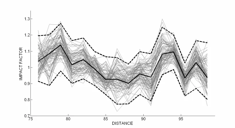
Figure 6 Distribution of spring stiffness, k: true (histogram) and fitted (___₎ Figure 7 Observed impact factors with predicted mean (____) and 95% prediction

limits (----) for the fitted model

Figure 8 Predicted impact factors for final 6 sensors with predicted mean (____) and 95% prediction limits (----)

0.8 0.85 0.9 0.95 1 1.05 1.1 1.15 1.2

0 2 4 6 8 10 12 14 16 18

Distance along Pavement (m)

IF

Type1 Type2 Type3 Type4 Type5 Type6 Type7 Type8 Type9

Table 1 – Means and standard deviations of vehicle suspension parameters, velocities and lateral approach positions

Parameter Unit Mean St. Dev.

Suspension Parameters Sprung Mass m2 kg 4450 445

Unsprung Mass m1 kg 420 -

Suspension Stiffness k N/m 500 x 103 _{50 x 10}3

Tyre Stiffness kt N/m 1950 x 103 195 x 103

Suspension Damping cb Ns/m 20 x 103 -

Approach Parameters Velocity v m/s 23.43 2.08

Lateral Approach Position z m 1.50 0.5

Gaussian noise in observed measurements of IF

2 _0.2