Studies on the Mixing in a Density Stratified Shear Flow

(1)

DENSITY-STRATIFIED SHEAR FLOW

by

Gregory Gartrell, Jr.

Thesis Supervisor: Norman H. Brooks James Irvine Professor of Environmental and Civil Engineering

Supported by

National Science Foundation

Grant Numbers GK35774X, ENG75-02985, ENG77-27398 Principal Investigator:

E. John List

Professor of Environmental Engineering Science

W. M. Keck Laboratory of Hydraulics and Water Resources Division of Engineering and Applied Science

California Institute of Technology Pasadena, California

(2)

ACKNOWLEDGMENTS

There are so many people to whom I owe so much, I feel I could write another volume the size of this one and still not thank everyone adequately. There are several friends who have been especially helpful over the last few years, and who have contributed to this work in many vital ways; I am sincerely grateful for the time, effort and friendship

these people have offered me.

The two people to whom I owe the most are Professors Norman H. Brooks and E. John List. Dr. Brooks, my principal advisor on this project,

suggested the topic and provided patient guidance and understanding as the work progressed. His warm sense of humor brightened countless days for me, and he always provided encouragement when it was needed.

Dr. List has been especially helpful. He has provided encouragement and friendship, and has always been willing to share a few moments to discuss new ideas and provide helpful insights. I owe more than I can ever repay to these two friends.

I would especially like to thank Elton Daly, whose special genius has never ceased to amaze me. No matter what needed to be built in the laboratory, Elton always had a better, simpler way to do it. He has been a close friend and an inspiration to me.

(3)

Professor Vito A. Vanoni deserves special thanks for the time and help he provided. His awesome dedication and vitality acted as a constant encouragement.

Joan Mathews typed a seemingly endless thesis, and retyped the

corrected versions, a Sisyphean task. She provided friendship throughout the past years, and kind encouragement when it was greatly needed the last few weeks. I am truly thankful.

During the sunnner of 1977, I participated in the Geophysical Fluid Dynamics Program at the Woods Hole Oceanographic Institution. My visit there as a pre-doctoral fellow provided me with the opportunity not only to meet with many interesting and knowledgeable people, but also to take some time to reflect on this research and to hear fresh ideas. I

returned from Woods Hole with a deeper understanding of the subject, and an enthusiasm that has stayed with me to this day. I would like to thank the Woods Hole Oceanographic Institution and the Geophysical Fluid Dynamics Program for the support they provided. I would also like to thank Professor George Veronis, who directed the program, and

Professor ~rten T. Landahl, with whom I had many worthwhile discussions, and who taught me so much about the subject of turbulence.

No one can conduct an experimental program alone, and in this instance I had valuable help from Joe Fontana, Rich Eastvedt and Dave Byrum. The fine talents of Joe Fontana and Rich Eastvedt turned rough sketches into apparatus that not only worked as intended, but also

(4)

than he or I would ever care to see again.

I would also like to thank Phil Cormier, who helped take data and who, along with Dale Ota, helped in the data reduction. This research could never have been completed without the signal processor for the laser-Doppler system. Marc Donner designed and built the first working model. I would also like to thank Larry McClellan and Catharine van Ingen

for their help.

There are several others who provided friendship, advice and assist-ance. I would especially like to thank Jim Pankow, Steve Wright, Phil Roberts, Jacques Lewalle and Jing-Chang Chen. I want to thank Mary Eichbauer for her love and encouragement and patience. I hope I can give as much as she continues with a task similar to this one.

I would like to thank the California Institute of Technology for providing facilities which made this study possible, and the National Science Foundation for providing financial support under Grants

GK35774X, ENG75-02985, ENG77-27398; the Environmental Protection Agency under Grant T-900137; the National Institutes of Environmental Health Science under Training Grant 5T01 ES00004-15 and the Ford Motor Company Fund/Ford Energy Research Program.

(5)

ABSTRACT

The objective of this study was to examine in a fundamental way the mixing processes in a stably stratified shear flow. The results of the experimental program have yielded information on the nature of turbulence and mixing in density-stratified fluids. The results can be applied to such problems as the determination of the spreading and mixing rates of heated effluents discharged to lakes or the ocean, as well as to many geophysical problems.

An experimental investigation was made to measure the mixing in a two-layered density-stratified shear flow in a flume 40-meters long, with a cross-section of 110 cm wide by 60 cm deep. Both mean tempera-tures and the mean velocities of the two layers could be independently controlled, and steps were taken to ensure that the temperatures and velocities of the two layers remained nearly constant at the inlet. The relative density difference between the layers was 10- 3 or less. A laser-Doppler velocimeter, designed for this study, allowed measure-ments of two components of velocity simultaneously, while a sensitive thermistor was used to measure the temperature. The temperature and velocity measurements were recorded and later analyzed.

The initial mixing layer which developed at the inlet was found to be dominated by large, two-dimensional vortex structures. When the flow was sufficiently stratified, these structures would collapse in a short distance and the flow would develop a laminar shear layer at the interface. It was found that the bulk-Richardson number

6

P giT*/6u 2, where i

* is the maximum-slope thickness of the

p o T

(6)

temperature profile, attained a maximum value between 0.25 and 0.3 when the mixing layer collapsed.

Downstream, much less turbulent mixing took place in the stratified flows than homogeneous flows. The depth-averaged turbulent diffusivities for heat and momentum were of ten 30 to 100 times smaller in stratified flows than in homogeneous flows. The turbulence downstream was found to be dominated by large turbulent bursts, during which the vertical turbulent transport of momentum, heat and turbulent kinetic energy are many times larger than their mean values. It was found these bursts were responsible for most of the total turbulent transport of momentum, heat and turbulent kinetic energy, even though the bursts were found only intermittently.

The flux-Richardson number, Rf' in the flow was examined and found to be related to the local mean-Richardson number in many cases. When

- - a u production of turbulent kinetic energy from the mean shear, -u'v' ay , was the largest source of turbulent kinetic energy, it was found that Rf

<

0.3, and when the

diffusion of turbulent

flow was strongly stratified, Rf

<

1 a(u'2

+

v'

2

_)v'

kinetic energy

2

ay

=

0.2. I f the was the largest source of turbulent kinetic energy, then the flux-Richardson number often attained large values, and the quantity - - ;aq*-p'v'g - 2v'

- - ay

Po

It was found that, in was found to be a more useful parameter than Rf.

(7)

TABLE OF CONTENTS

ACKNOWLEDGMENTS ABSTRACT

TABLE OF CONTENTS LIST OF FIGURES LIST OF TABLES NOMENCLATURE CHAPTER 1 CHAPTER 2

INTRODUCTION

THEORETICAL ANALYSIS AND REVIEW OF PREVIOUS WORK 2.0 Introduction

2.1 Equations of Motion and Pertinent Dimensionless Quantities

2.1.1 Equations of Motion 2.1.2 Dimensionless Parameters

2.2 Stability Considerations for Stratified Shear Flows

ii v vii xv xxvii xx ix

1 5 5

6

9

14 2.3 Turbulent Mixing With Buoyancy Effects 30 2.4 Spectral and Other Properties of Turbulent Flows 35

2.4.1 Spectral Considerations 35

2.4.2 Coherent Structures in Turbulent Fields 38

2.5 Integral Balances 40

2.6 Initial Mixing Layer 42

2.7 A Review of Experiments on Mixing in

(8)

CHAPTER 3

2.7.1 Entrainment Rates in Stratified Fluids--Shear Flow Experiments 2.7.2 Entrainment Rates in Stratified

Flows--Oscillating Grid Experiments 2.7.3 Turbulent Diffusivities in Stratified

Flows

2.7.4 Qualitative Observations of Stratified Flows

EXPERIMENTAL APPARATUS 3.0 Experimental Objective 3.1 Flume Characteristics

3.2 Heating and Cooling of the Water 3.3 Temperature Measurements

3.4 Velocity Measurements 3.5 Laser-Doppler Carriage 3.6 Data Acquisition System CHAPTER 4 EXPERIMENTAL PROCEDURE

4.0 Introduction

4.1 Instrument Calibration and Usage

45 49 53 55 61 61 61 67 69 74 88 91 95 95 95

4.1.1 Thermistors 95

4.1.2 Laser-Doppler Velocimeter Calibrations 97 4.1.3 Error Analysis for the Laser-Doppler

System

4.1.4 Venturi Meters

4.1.5 Depth and Slope Measurements

(9)

CHAPTER 5

CHAPTER 6

4.1.6 Density Measurements 4.2 Boundary Heat Losses

4.3 Experimental Procedure

4.4 Errors in Velocity Measurements Due to Thermal-Optical Effects

4.4.1 Effects of the Mean Temperature Gradient

4.4.2 Errors Due to Fluctuations in the Refractive Index

4.5 Data Analysis

GENERAL DESCRIPTION OF THE FLOW 5.0 Introduction

5.1 Inlet Conditions

5.1.1 Splitter Plate Wake

5.1.2 Inlet Turbulence Levels and Flow Uniformity

5.1.3 Inlet Temperature Profile

5.2 Bottom Roughness and Boundary-Generated Turbulence

5.3 Qualitative Flow Description I -The Initial Mixing Layer

5.4 Qualitative Flow Description II -Downstream Mixing and Instabilities PRESENTATION OF EXPERIMENTAL RESULTS 6.0 Introduction

(10)

6.1 Experimental Parameters 199 6.2 Experimental Results from Measurements in

the Initial Mixing Layer 203

6.2.1 Profiles of the Mean Horizontal

Velocity 206

6.2.2 Profiles of the Mean Temperature 210 6.2.3 Growth Rates and Length Scales in

the Mixing Layer 213

6.2.4 Collapse of the Mixing Layer 219 6.2.5 Profiles

of~

u' 2,

~

v' 2

and~

T'2 225 6.2.6 Profiles of Turbulent Flux Quantities 235 6.2.7 Probability Density Functions of

Fluctuating Quantities 248

6.2.8 Power Spectral Estimates of

6.2.9 Integral Balances 265

6.2.10 Turbulent Energy Exchange 270 6.2.11 Sunnnary of the Results for the Initial

Mixing Layer 280

6.3 Experimental Results from Measurements Made

in the Downstream Flow Over a Smooth Bed 281 6.3.1 Profiles of Mean Velocity and

Temperature 282

(11)

6.3.3 Properties of

~

T' 2, -v'T' and u'T' 293 6.3.4 Power Spectral Estimates of

6.3.5 Turbulent Energy Exchange 306 6.3.6 Summary of the Results for the

Downstream Flow Over a Smooth Bed 310 6.4 Experimental Results from Measurements Made in

the Downstream Flow Over a Roughened Bed 311

6.4.1 Profiles of Mean Velocity and Temperature 312 6.4.2 Profiles of

~

u' 2,

~

v' 2 and -u'v' 318 6.4.3 Profiles

of~

T'2 and -v'T' 325 6.4.4 Power Spectral Estimates of Fluctuating

Quantities 327

6.4.5 Turbulent Energy Exchange 331

6.4.6 Summary of the Results for the Downstream Flow Over a Roughened Bed 347 6.5 Organized Structures in the Turbulent Regions 349

6.5.1 Probability Density Functions in

Turbulent Regions 350

6.5.2 Time-Records of Fluctuating Quantities 366 6.5.3 Mean Quantities from Conditionally

Sampled Data Records 379

6.5.4 Summary of the Results on Organized

(12)

CHAPTER 7 DISCUSSION OF THE EXPERIMENTAL RESULTS 7.0 Introduction

7.1 Discussion of the Results of the Measurements in the Initial Mixing Layer

7.1.1 Comparison of Measured Profiles and the Gross Features of the Initial Mixing Layer

7.1.2 Growth and Collapse of the Stratified

Page 391 391

391

Mixing Layer--Macroscale Measurements 402 7.1.3 Growth and Collapse of the Stratified

Mixing Layer--Energy Exchange 7.1.4 Summary of the Discussion on the

Initial Mixing Layer

7.2 Turbulent Energy Exchange Processes 7.2.1 Conservation Equations for

407

413 415

7.2.2 Turbulent Energy Exchange Relationships 422 7.2.3 Sunnnary of the Discussion on Turbulent

Energy Exchange Processes

7.3 Discussion on Coherent Structures in the Turbulent Flow

7.3.1 Comparison with the Findings in

426

427

Other Studies 428

(13)

CHAPTER 8 SUMMARY AND CONCLUSIONS 437

REFERENCES 441

APPENDIX

A A

Signal Processor for a Laser-Doppler Velocimeter (previous publication, by Gregory Gartrell~ Jr.; available under a separate cover as Tech. Memo. 78-5, W. M. Keck Laboratory of Hydraulics and Water

(14)

[image:14.593.96.517.120.724.2]

Figure 2.2.1 2.2.2 2.2.3 2.2.4 3.3.1 3.1.2 3.1. 3 3.3.1 3.3.2 3.3.3 3.3.4 3.3.5 3.3.6 3.3.7 3.4.1 3.4.2 3.4.3 3.4.4 3.4.5 3.4.6 3.4.7 3.4.8

LIST OF FIGURES Description

Breakdown due to focusing of a secondary wave Assumed velocity and density profiles for model Regions for solutions in Ri - k space

1 Wave trapping condition for c =

2

The 40-m flume used for experiments Flume outlet hoppers

Flume inlet hopper

Photograph of a glass-bead thermistor Glass-bead thermistor circuit

Rake of eight thermistors Array of ten thermistors

Photograph of a fast-response thermistor Fast-response thermistor circuit

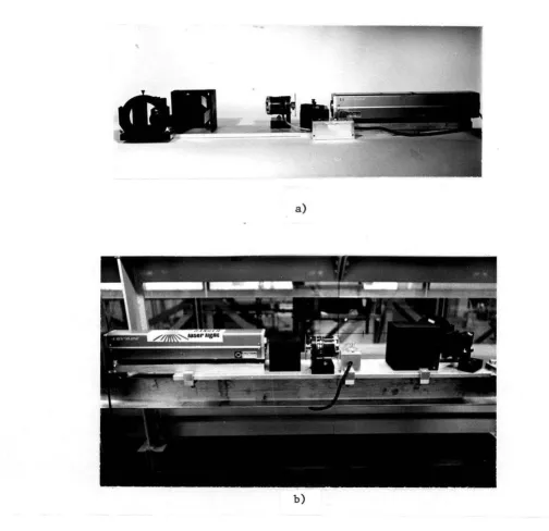
Transfer function for fast-response thermistor Reference beam system for laser-Doppler velocimeter Optical arrangement for laser-Doppler velocimeter Photograph of the laser-Doppler velocimeter

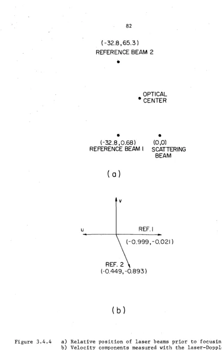
Beam positions and velocity components measured by the laser-Doppler velocimeter

Laser-Doppler signal, background noise channel 1 Laser-Doppler signal, background noise channel 2 Laser-Doppler signal, background noise channels 1 and 2

Laser-Doppler signal during operation channel 1

(15)

Figure 3.4.9 3.5.1 3.6.1 4.1.1 4.1.2 4.1.3 4.1.4 4.1.5 4.4.1 4.4.2 4.4.3 4.4.4 4.4.5 4.4.6 4.4.7 4.4.8 4.4.9 4.4.10 Description

Laser-Doppler signal during operation channel 2 Photograph of the carriage for the laser-Doppler velocimeter

Buffer circuit for the A/D converter

Typical calibration curve for the glass-bead thermistors

Typical calibration curve for the fast-response thermistor

Size distribution of particles in the flow Flow rate calibration, Venturi meter Q-6 Flow rate calibration, Venturi meter Q-39

Comparison of u profiles for a homogeneous flow and a stratified flow

Comparison of

~

u' 2 and

~

v' 2 profiles for a homogeneous flow and a stratified flow

Comparison of -u'v' profiles for a homogeneous flow and a stratified flow

Comparison of

~T'

2

profiles for a homogeneous flow and a stratified flow

Comparison of spectra for u' for a homogeneous flow and a stratified flow

Comparison of spectra for v' for a homogeneous flow and a stratified flow

Smoothed spectra from Figure 4.4.5

Power spectra for u', v' and T' in a laminar region of a strongly stratified flow

Power spectra for u', v' and T' in a turbulent region of a strongly stratified flow

Power spectra for u', v' and T' in a weakly stratified flow

(16)

Figure 4.5.1 4.5.2 5.1.1 5.1.2 5.1.3 5.1.4 5.1.5 5.1.6 5.1. 7 5.1.8 5.1.9 5.1.10 5.1.11 5.1.12 5.2.1 5.2.2 5.2.3 5.2.4 5.2.5 5.2.6 Description

Time-records for u' and T' in a strongly stratified flow

Filtered velocity record from Figure 4.5.l Profile of;;, x

=

0.1 m,

Profile of u, x = 0.2 m, Profile of u, x

=

0.2 m, Profile of u, x = 0.4 m, Profile of u, x = 4.7 m,

LiU

=

6 cm/s

0

LiU

=

6 cm/s

0

LiU

=

3.6 cm/s

0

LiT

=

1.5°C

0

LiT

=

1.4°C

0

Photograph of a vertical dye streak at the inlet, LiU ~ -0.5 cm/s

0

Photograph of a vertical dye streak at the inlet, LiU ~ 6 cm/s

0

Profiles

of~

u'2 and

~

v'2 at x = 0.2 m Profile of -u'v' at x

=

0.2 m

Photographs of dye streaks across the flume channel at the inlet

Profiles of T and

~T'

2 at the inlet Isotherms at the flume inlet

Profile of u'v' at x

=

21.5 m, smooth bed, homogeneous flow

Profiles

of~

u'2 and

~v'

2

at x

=

Profile of u at x

=

Power spectra of u' and v' at x = 21.5 m, smooth bed, homogeneous flow

Arrangement of bricks on the flume bed

Profile of u, x = 24 m, brick-roughened bed, homogeneous flow

(17)

Figure 5.2.7 5.2.8 5.2.9 5.2.10 5.2.11 5.2.12 5.2.13 5.2.14 5.3.la 5.3.lb 5.3.2a 5.3.2b 5.3.2c 5.3.3a 5.3.3b 5.3.3c 5.4.1 5.4.2 Description

Profiles of

~

u' 2. and

~

v' 2., x

=

24 m, brick-roughened bed, homogeneous flow

Profile of -u'v', x = 24 m, brick-roughened bed, homogeneous flow

Power spectra of u' and v' at x

=

24 m, brick-roughened bed, homogeneous flow

Photograph of the rock-roughened bed

Profile of u, x = 24 m, rock-roughened bed, homogeneous flow

Profiles of

~u'

2 and~

v'2 , x = 24 m, rock-roughened bed, homogeneous flow

Profile of -u'v', x = 24 m, rock-roughened bed, homogeneous flow

Power spectra of u' and v', x

=

24 m, rock-roughened bed, homogeneous flow

Photographs of the mixing layer, x

=

0.3 m Photographs of the mixing layer, x

=

1.05 m Photographs of the mixing layer, x = 0.3 m Photographs of the mixing layer, x

=

1.05 m Photographs of the mixing layer, x

=

1.8 m Photographs of the stratified mixing layer,

x = 0.3 m

Photographs of the collapsing mixing layer, x = 1.8 m

Photographs of the collapsing mixing layer, x = 2. 6 m

Photograph of vertical dye streaks in a stratified flow, x

=

15 m, smooth bed

Photographs of a dye streak in a stratified flow, x

=

15 m, smooth bed

(18)

Figure 5.4.3 5.4.4 5.4.5 5.4.6 5.4.7 5.4.8a 5.4.8b 5.4.9 6.2.1 6.2.2 6.2.3 6.2.4 6.2.5 6.2.6 6.2.7 6.2.8 6.2.9 6.2.10 Description

Photographs of vertical streaks in a strongly stratified flow

Photographs of internal waves in a strongly stratified flow

Photographs of vertical dye streaks in a homogeneous flow, x = 15 m, smooth bed

Photographs of small waves breaking on a large internal wave; stratified flow x = 20 m

Photographs of a large internal wave breaking; stratified flow, x = 20 m

Photographs of small waves breaking in a stratified flow, x

=

20 m

Photographs of a large internal wave in a stratified flow, x = 20 m

Photographs of dye streaks across the flume channel, x

=

20 m

Normalized profiles of u in the initial mixing layer

Normalized profiles of u in the mixing layer, x/9.b > 4

Normalized profiles of T in the mixing layer Normalized profiles of T in the mixing layer, x/9.b

>

4

Growth rates of 9. * in the mixing layer

u

9.T*/9.b versus x/9.b in the mixing layer 9.T*/9.u* versus x/9.b in the mixing layer

(Ri) . versus x/9.h in the mixing layer min

11.p g 9. * / 11.u 2 versus x/ 9.b in the mixing layer

p

0 u o

k g 9. * / t::.u 2 versus x/ 9.b in the mixing layer

p T o

(19)

Figure Descri}2tion Page 6.2.11 Normalized profiles of

l

u' 2 in the mixing layer 226 6.2.12 Normalized profiles of

l

u' 2 in the mixing layer 228 6.2.13 Normalized profiles of

~

v' 2 in the mixing layer 229 6.2.14 Normalized profiles of

~

v' 2 in the mixing layer 231 6.2.15 Normalized profiles of

~

T' 2 in the mixing layer 232 6.2.16 Normalized profiles of

~

u'2, x/9.,b

>

4 233 6.2.17 Normalized profiles of

p,

x/.l!.b

>

4 234 6.2.18 Normalized profiles of

~

T'2, x/.l!.b

>

4 236 6.2.19 Normalized profiles of -u'v' in the mixing layer 237 6.2.20 Normalized profiles of -u'v' in the mixing layer 238 6.2.21 Correlation coefficients for u' and v' in the

mixing layer 240

6.2.22 Normalized profiles of -v'T' in the mixing layer 241 6.2.23 Normalized profiles of -v'T' in the mixing layer 242 6.2.24 Correlation coefficients for v' and T' in the

mixing layer 243

6.2.25 Normalized profiles of -u'v'

'

x/.l!.b

>

4 245

6.2.26 Correlation coefficients for u' and v', x/.l!.b

>

4 246 6.2.27 Normalized profiles of -v'T' x/.l!.

>

4

' b 247

6.2.28 Normalized profiles of q*2u• in the mixing layer 249 6.2.29 Normalized profiles of q*2v' in the mixing layer 250 6.2.30 Probability density functions for v', stratified

mixing layer 252

6.2.31 _{Probability density functions for u'' homogeneous}

mixing layer 253

6.2.32 Probability density functions for u 'v', stratified

(20)

[image:20.593.96.530.100.705.2]

Figure 6.2.33 6.2.34 6.2.35 6.2.36 6.2.37 6.2.38 6.2.39 6.2.40 6.2.41 6.2.42 6.3.1 6.3.2 6.3.3 6.3.4 6.3.5 6.3.6 6.3.7 6.3.8 6.3.9 6.3.10 Description

Probability density functions for u'v', homogeneous mixing layer

Probability density functions for v'T', stratified mixing layer

Probability density functions for v', collapsing mixing layer

Probability density functions for u'v', collapsing mixing layer

Probability density functions for v'T', collapsing mixing layer

Power spectra for u' and v', homogeneous mixing layer

Power spectra for u', v' and T', stratified mixing layer

Power spectra for u', v' and

T',

stratified mixing layer

Rf versus Ri, in the initial mixing layer

- - *

_{B'v'/£ versus}

-

_Ri, _{in the initial mixing layer}

Profiles of u, x

=

4.7 m, Experiments BH6,BH7,B4 Profiles of u, x = 21.4 m, Experiments BH6,BH7,B4 Profiles of T, x = 4.7 m, Experiments BH6,BH7 Profiles of T, x = 21.4 m, Experiments BH6,BH7 Profiles of u, x = 4.7, Experiments BH14,BH15 Profiles of u, x = 20 m, Experiments BH14,BH15 Profiles of T, x = 20 m, Experiments BH14,BH15 Profile of

u, x

=

24 m, Experiment BH16

Profile of T, x

=

24 m, Experiment BH16

Profiles

of~

u'2 , x

=

4.7 m, Experiments BH6,BH7,B4

(21)

[image:21.595.94.528.105.726.2]

Figure 6.3.11 6.3.12 6.3.13 6.3.14 6.3.15 6.3.16 6.3.17 6.3.18 6.3.19 6.3.20 6.3.21 6.3.22 6.3.23 6.3.24 6.3.25 6.3.26 6.3.27 6.4.1 6.4.2 6.4.3 6.4.4 6.4.5 Description

Profiles

of~

v'2 , x = 4.7 m, Experiments BH6,BH7,B4 Profiles of -u'v', x = 4.7 m, Experiments BH6,BH7,B4 Profiles of

~u'

2

,

x = 21.4 m, Experiments BH6,BH7,B4 Profiles

of~

v'2 , x

=

21.4 m, Experiments BH6,BH7,B4 Profiles of -u'v', x

=

21.4 m, Experiments BH6,BH7,B4 Profiles

of~

v'2 , x = 20 m, Experiments BH14,BH15 Profiles of -u'v', x = 20 m, Experiments BH14,BH15 Profiles of

~T'

2

,

x = 20 m, Experiments BH14,BH15 Profiles

of~

T'2 , x = 24 m, Experiment BH16

Profiles of -v'T', x

=

20 m, Experiments BH14,BH15 Profile of ~v'T', x = 24 m, Experiment BH16

Power spectra of u', v' and T' in a stratified flow Power spectra of u', v' and T' in a laminar region of a stratified flow

Power spectra of u', v' and T' in an intermittently turbulent region of a stratified flow

Power spectra of u', v' and T' in a turbulent region of a stratified flow

Rf versus Ri from measurements in the downstream flow over a smooth bed

B'v'/E* versus Ri, from measurements in the downstream flow over a smooth bed

Profiles of u, x = 20 m, Experiments CH4,C4 Profiles of

u,

x

=

24 m, Experiments D5,DH5,DH7 Profiles of

u, x

=

24 m, Experiments DH6,DH7 Profiles of T, x = 24 m, Experiments DH6,DH7 Profiles of

~'

2

,

x

=

20 m, Experiments CH4,C4

(22)

Figure 6.4.6 6.4.7 6.4.8 6.4.9 6.4.10 6.4.11 6.4.12 6.4.13 6.4.14 6.4.15 6.4.16 6.4.17 6.4.18 6.4.19 6.4.20 6.4.21 6.4.22 6.4.23 6.4.24 6.4.25 6.4.26 Description

Profiles of -u'v', x = 20 m, Experiments CH4,C4 Profiles of

~u'

2

,

x

=

24 m, Experiments D5,DH5,Dh7 Profiles of

~v'

2

,

x = 24 m, Experiments D5,DH5,DH7 Profiles of -u'v', x = 24 m, Experiments D5,DH5,DH7 Profiles of

~u'

2

,

x

=

24 m, Experiments DH6,DH7 Profiles of

~v'

2 ,

x

=

24 m, Experiments DH6,DH7 Profiles of -u'v', x

=

24 m, Experiments DH6,DH7 Profiles

of~

T'2 , x = 24 m, Experiments DH6,DH7 Profiles of -v'T', x = 24 m, Experiments DH5,DH7 Profiles of -v'T', x

=

24 m, Experiments DH6,DH7 Power spectra of u', v' and T' in an intermittently turbulent region of a stratified flow

Power spectra for u', v' and T' in a turbulent region of a stratified flow

Rf versus Ri, in weakly stratified, turbulent flows Rf versus Ri in strongly stratified, turbulent flows

IE*I

<

0.5

Profiles of turbulent energy quantities from Experiment DH7, x = 24 m

Rf and B'v'/£* versus Ri, Experiment DH7, x Rf versus E*, for E*

>

1

*

~

*

F = Rf/E versus Ri, for E

>

1

24 m

B'v'/£* versus Rf, in weakly stratified turbulent flows

(23)

Figure Description Page 6.4.27 B'v' ff;* versus Ri, for E* > 0.6 346 6.5.1 Probability density functions for u' and v',

Experiment DH6 351

6.5.2 Probability density functions for u', Experiment DH6 353 6.5.3 Probability density functions for v', Experiment DH6 354 6.5.4 Profiles of

~

u'2 ,

~

v'2 and u'v' for Experiment DH6 355 6.5.5 Probability density function for u'v', Experiment DH6 357 6.5.6

r

(L) and <u'v'> /u'v' (L) versus LP 359

p

6.5.7 Probability density functions for u'v', Experiment DH6 360 6.5.8 Probability density functions for u'v', Experiment DH6 361 6.5.9 Probability density functions for v'T', Experiment DH6 363 6.5.10 Probability density functions for v'T', Experiment DH6 364 6.5.11 Probability density functions for v'T', Experiment DH6 365 6.5.12 Time-records of fluctuating quantities, Experiment CH3 368 6.5.13 Time-records of fluctuating quantities, Experiment D5 370 6.5.14 Time-records of fluctuating quantities, Experiment D5 372 6.5.15 Time-records of fluctuating quantities, Experiment DH6 373 6.5.16 Time-records of fluctuating quantities, Experiment DH7 375 6.5.17 Time-records of fluctuating quantities, Experiment DH7 376 6.5.18 Time-records of fluctuating quantities, Experiment B4 377 6.5.19 Conditionally sampled averages for u'v', Experiment CH4 382 6.5.20 Conditionally sampled averages for u'v', Experiment CH3 385 6.5.21 Conditionally sampled averages for u'v' and v'T',

Experiment CH3 385

(24)

Figure 6.5.23 6.5.24 7 .1.1 7 .1. 2

7 .1.3

Description Mean time between bursts versus L

c

Mean time between one-sided bursts versus L c Graphic depiction of the initial mixing layer Bulk-Richardson number versus Ri, from several investigations

Turbulent energy quantities from the initial mixing layer versus x/tb

389

401

403

(25)

Table 3.3.1 3.4.1 4.1.1 4.1. 2

6.1.1 6.1.2 6.1.3 6.1. 4 6.2.1 6.2.2 6.2.3

LIST OF TABLES

Thermistor characteristics Laser-Doppler velocimeter data

Data for Equations 4.5.la and 4.5.lb Estimated probable errors for velocity measurements

Parameters for experiments with homogeneous flow Mixing layer experiments

Smooth bed experiments, downstream measurements Roughened bed experiments, downstream measurements Centerline flow speed for mixing layer experiments Mixing layer growth rates

Measured quantities for integral balances of mass, momentum and buoyancy

69 83 103

108 200 201

2al

202 205 215

(26)

A B E F G 1,1* K u K m L L c L p N p NOMENCLATURE constant

buoyant force per unit mass, constant

constant constant

aq2v ' / - - au _u'v'

-ay ay

aq*

2

v'/--au

- u'v'

-ay ay

--/aq

2_v'

-B'v' -ay

p-p 0

g

p

₁

p~

1

_/

2 _{(Section 2.2, Equation 2.2.7)}

conditional sampling functions (Section 6.5.3,

p 0

0

Equations 6.5.3, 6.5.4) Keulegan number, v

~P

go/iu 3

turbulent diffusivity of momentum,

-u'v'/~;

turbulent diffusivity of heat, -v'T'/aT

ay path length of laser beam

conditional sampling level (Section 6.5.3, Equation 6.5.3) conditional sampling level (Section 6.5.1, Equation 6.5.1)

- 1/2

(27)

p _r

*

R c

R

*

c Re Ri Ri

s

T T 0

u

turbulent Prandtl number Km/~

total volumetric flow rate

total volumetric flow rate of the upper layer total volumetric flow rate of the lower layer bulk-Richardson number bp gt/bU 2

p 0

0

( 1 + _v'2Q2" t l ) ₂ _t2

.,-1

-1

(1

+

2q*2

:1

*)

v' 2 2

Reynolds number, 4~U/v

I

-- -- -- -- au flux-Richardson number

-B'v'

u'v' ay

hydraulic radius, wfh/(wf

+

2h)

Richardson number

I

2

2£.

au -g ay ( ay)

mean-Richardson number surface slope of flow temperature

constant, reference temperature

initial temperature of the upper layer initial temperature of the lower layer Tl - Tz

total mean flow speed, Q/wfh

(28)

LiU 0

v

0 LiV c c g f f f p g h voltage

reference voltage

estimated error in voltage measurements

phase speed of a wave group velocity of a wave constants (Section 2.4)

unit vector in the direction of reference beam unit vector in the direction of scattering beam friction factor

Section 2.2, amplitude of G frequency

acceleration due to gravity, in the negative y(x

2) direction total flow depth

initial depth of the upper layer

initial depth of the lower layer, 30 cm current from photomultiplier tube

wave number length scale

c\11

+

u-2

>/Af!..

buoyancy length scale, liu

0 2 P g

0

integral length scale for temperature (Equation 2.1.21) maximum-slope thickness of temperature profile

(29)

JI,

*

u n p t -~ th' th tl t2 t

*

2 t3 u u e v w

maximum-slope thickness of the velocity profile (Equation 2.1.19)

displacement thickness (Equation 5.1.1) index of refraction

_lg_ =

..2.£... -

~

pressure, ax.

ox.

pogui2

l. l.

probability density function 1 (u'2

+

v'2

+

w'2)

2

1

2

time

mean period between bursts (Section 6.5.3) p'2/2£p

q2/£

q2f£

P

'v'

_{/£ pv}

velocity component in x-direction entrainment velocity

velocity component in the ith direction

initial mean centerline speed of the upper layer initial mean centerline speed of the lower layer ul - u2

shear velocity

velocity component in the y~direction

(30)

x x c

*

x c

x.

1 y z a a* y 0 •. 1J

0 I

w £

c.*

£ pv

e

K A m

distance in the horizontal direction of the mean flow distance to the collapse of the large structure

in the initial mixing layer x/9-b

distance in the ith direction distance in the vertical direction

distance in the horizontal direction, transverse to the mean flow

parameter in Equation 2.2.2 d(p-p )/d(T-T )Ip

0 0 0

parameter, Section 2.2 Kronecker delta function

d(R, *) u d x

a.2

=

k2

+

""4"" -

ga/c2

dissipation rate per unit mass of the turbulent kinetic energy, q2

dissipation rate per unit mass for q* 2 dissipation rate for p'2/2

dissipation rate for p'v'

fluid particle displacement (Section 2.2) k(x - ct) (Section 2. 2)

thermal diffusivity

(31)

µ \)

"n

\) m p cr p " cr s (J u

(J I

u

CJ I

v

*

-r,r ,r

x

qi 'qi 'qiT(k) _u _v

qi*(f ) p

dynamic viscosity

kinematic viscosity, µ/p Doppler frequency

relative error in Doppler frequency measured value of "D

fluid density

constant, reference density

perturbation in density, Section 2.2

initial relative density difference between the upper and lower layers (positive)

probable relative error in repeatability systematic relative error

a _u

'/u

error estimate for u cr '/u _v

error estimate for v

amplitude of 1jJ (Section 2.2)

time fraction for turbulent bursts (Section 6.5.3, Equations 6.5.1 - 6.5.8)

dissipation rate for T'2

stream function of perturbation wave (Section 2.2)

power spectral estimates for u', v' and T' where qi=~ qi* 21T and k = 21Tf

/u

p

(32)

E

UV

E qv

prime (' ) overbar (

[

<

>

i,j ,k

standard deviation of u'v' record standard deviation of q* 2v' record

SPECIAL NOTATION

fluctuating part of a quantity (e.g. u' = u - u) ) mean value of a quantity

normalization such that the mean is zero and the standard deviation is one

conditionally sampled average (Section 6.5.3, Equations 6.5.1 - 6.5.8)

SUBSCRIPTS integer indices

(33)

CHAPTER 1 INTRODUCTION

Density-stratified shear flow problems are commonly encountered both in engineering practice and in geophysical studies. Yet, as with many fluid mechanics problems, they are not well understood. Part of the reason for this is that solutions for density-stratified shear flow problems of ten require some knowledge of the behavior of turbulence in fluids, at best a complicated and poorly understood matter. There are, however, a number of vital engineering problems which require knowledge on a fundamental level concerning the behavior of density-stratified shear flows in order that they might be intelligently solved.

Among these problems is that of the discharge of cooling water from power plants to lakes or the ocean. In such instances, a buoyant layer of warm water may form on the surface and slowly spread. The rate at which this layer of water drifts over and mixes with the cooler ambient water will depend upon, among other things, the density differ-ence between the two layers, the shear at the interface, and the

turbulence levels in the vicinity of the interface.

Another related problem is that of the discharge of sewage to the ocean; whether the sewage field rises to the surface or stays submerged, the ultimate turbulent mixing processes involve interactions with

(34)

density-stratified shear flow problems. In addition, there are many geophysical stratified flow problems. These include atmospheric

motions, the nature of oceanic currents, and the behavior of estuarine flows. There are also many problems related to mixing in lakes and reservoirs which involve density stratification.

The purpose of this study is to examine in detail the mixing which takes place in a two-layered density-stratified turbulent shear flow. The ultimate goal is to provide fundamental information on the nature of such flows in order that one might have a better understanding of them when approaching engineering problems.

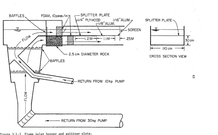
As a major part of this study, an experimental investigation was conducted in order to measure the mixing in a density-stratified shear flow. Experiments were conducted in the 40-meter precision tilting flume in the Keck Hydraulics Laboratory. The flume was modified so that at the upstream end warm water entered the flume at one velocity from above a splitter plate, while cooler water entered at a slower velocity from below. At the downstream end, an adjustable splitter plate separated the upper and lower layers of water which were then

returned to the inlet via separate return pipes with temperature control. Velocity measurements were made using a two-component laser-Doppler

velocimeter, developed for this study, while temperature measurements were made with sensitive thermistors. The results of the measurements have yielded much new information on the nature of density-stratified flows.

(35)

theoretical vein in order that the results of the experimental investi-gation might be more easily understood. Together, the theoretical and experimental investigations have answered a number of questions about the nature of density-stratified shear flow problems, but leave many more questions still unanswered.

Chapter 2 presents a review of some previous experimental and

theoretical work related to density-stratified shear flows. In addition, new theoretical work is presented, including some work which was con-ducted by the author at the Geophysical Fluid Dynamics Program at the Woods Hole Oceanographic Institution.

Chapter 3 contains a discussion of the experimental apparatus. Included is a detailed description of the laser-Doppler velocimeter used in the study. (Appendix A contains a detailed description of the electronics used with the laser-Doppler velocimeter.)

In Chapter 4 the experimental procedure. is described. Included are accounts of the calibration procedures of the various instruments and analyses of the measurement errors. Also included is a discussion on possible errors in velocity measurements caused by variations in the refractive index of the water in the density-stratified flows.

Chapter 5 contains a general description of the flow. Included are discussions on the inlet conditions and the boundary-generated turbulence. In addition, some results from flow visualization studies are presented.

(36)

layer, the downstream flow over a smooth bed, the downstream flow over a roughened bed, and the organized structures found in the turbulent regions.

(37)

CHAPTER 2

THEORETICAL ANALYSIS AND REVIEW OF PREVIOUS WORK

2.0 Introduction

In this chapter previous theoretical and experimental studies on density-stratified shear flows are reviewed and some new analysis is presented. As discussed in Chapter 1, the bulk of this study concerns the experimental investigation of the mixing between a warm layer of water flowing over a colder layer. There are four basic regimes of mixing in this type of flow. The first regime is the initial two-dimensional mixing layer, which, given a sufficiently large buoyancy difference between the layers, can collapse to a laminar shear layer. If the mixing layer does not collapse, then downstream the fluid con-tinues to mix due to boundary-generated turbulence, although it mixes at rates which are much lower than those found in homogeneous open-channel flows. This is the second mixing regime.

The third and fourth regimes are closely related and occur down-stream if the mixing layer has collapsed. Shear stresses at the boundary of the flume may alter the velocity profile in such a way that a strong shear will exist across the stable interface. In

(38)

turbulence "chips" away at the lower portion of the interface, without totally disrupting the interface.

The balance of this chapter considers theoretical analyses and experimental work which relate to these types of mixing processes. Of particular interest are studies relating to mixing layers and the nature of turbulence in density-stratified shear flows.

2.1 Equations of Motion and Pertinent Dimensionless Quantities

In this section, the pertinent equations of motion and the impor-tant dimensionless quantities are presented and discussed. For con-venience, subscripted notation is used here; the variables and notation used are defined as follows: u. denotes the fluid velocity in the x.

1 1

direction, and (u

1,u2,u3)

=

(u,v,w), while (x1,x2,x3)

=

(x,y,z) where x is in the direction of the mean flow, y is in the vertical direction and z is in the lateral direction. An overbar (~) denotes an ensemble average and a prime (') denotes the usual fluctuating quantity. µ denotes the dynamic viscosity, p the density and v

=

µ/p, the kinematic viscosity; P denotes the pressure, T denotes temperature, and t denotes time.

2.1.1 Equations of Motion

The flow is assumed to be incompressible, hence, the continuity equation:

au.

1

axi = 0 .

In addition, a linear equation of state, p - p

0

(2.1.1)

= a1~ (T - T ) , valid

(39)

for small temperature differences, is assumed, so that

(2.1.2)

where K is the thermal diffusivity coefficient,

Po is a reference density, and T is a reference temperature.

0

The momentum (Navier-Stokes) equation is given by

(2.1.3)

where

o ..

is the Kronecker delta function, and g denotes the

accelera-1.J

tion due to gravity (in the negative x

2 direction). Following the work of Phillips (1966), Equation 2.1.3 can be reduced to

au . au. 1 a p-p 0 a 2u . "'ti + u.

"'x.1

= - - ~ - - -

go

+~ i

a .K a .K p axi p i2 p a~ a~ (2.1.4)

where and

P

0 is a constant, reference density.

The Boussinesq assumption (in which it is assumed that p ~ p , a constant,

0

except in the term involving the gravity force) is used and

au. au. 1 a a2u.

at

1

+

~

ax.1 = -

P-

1}- -

B 0 i2

+

v 1

.K ₀ ₁ a~a~

(40)

p-p

is obtained. Here B denotes the buoyant force per unit mass, ~-0- g. Po

From Equations 2.1.1 and 2.1.5, the following relationships can be derived (see Phillips (1966), Tennekes and Lumley (1972), Hinze (1959))

au. au. 1 "I

1 - 1 dTI

--+u.-=--~-Bo

at K ax. p ax. i2

K o 1

au. --1:. = 0

ax. _{]_}

2-au

'i·

u'k a u.

- - - + \) _ _

i _

a~ a~a~

au'. u'. _{]_} _J au. au. au'. u'. au'.u'.u'k

+

u

'k

u'j 1

+ ' '

_.J_

+

~

]_ J

+

]_ J

at a~ uiuk _a~ _a~ _a~

- ( u'j

2L_

+ '

;i; )/

P

0 - (

ujB'0 21

+

uj_B'Ozj)

2

a _x. u . ₁

_{- 3}

_°ij_e:

1

aB'2 + 2 ' B' at u k

and

(2.1.6)

(2.1.7)

(2 .1.8)

=

(2.1.9)

(41)

oB 'u'. au.

oB oB'u'. oB 'u' u'

].

+

B'u' _____!.

+

_{u 'i u 'k}

+~ ].

+

i k

at k _()~ _oxk _()~ _()~ =

- gEpu 1 _B'

2L_

_{B'2 0}

i2 (2.1.11)

Po

ox.

]. Po

Here E is the viscous energy dissipation rate per unit mass, E is the

p

dissipation rate for p' 2/2 and E is the dissipation rate for p'u.'.

pu J.

Equations 2.1.6, 2.1.7, and 2.1.8 are the conservation equations for the mean quantities of momentum, mass and buoyancy for a Boussinesq flow. Equations 2 .1. 9 - 2 .1.11 are conservation equations for second-order fluctuating quantities. For a detailed discussion of the terms in these equations, the reader is referred to Hinze (1959) or Tennekes and Lumley (1972).

From Equation 2.1.9, the conservation equation for turbulent kinetic energy is found to be

(2 .1.12)

where

These are the primary equations that are used in analysis of stratified shear flows.

2.1.2 Dimensionless Parameters

(42)

to describe density-stratified shear flows. One parameter is the Richardson number, Ri, which is defined as:

Ri

Clp

g

-ay

(2.1.13)

This quantity is useful in the analysis of laminar flows with wavelike perturbation; its usefulness in turbulent flows is open to question, since it is a rather difficult parameter to measure in a turbulent flow, and has both spatial and temporal fluctuations. The Richardson number is a stability parameter, for Miles (1961) and Howard (1961)

have shown that a sufficient condition for an inviscid density-stratified shear flow to be stable is that the Richardson number be everywhere greater than 1/4.

A more commonly used parameter in a turbulent density-stratified shear flow is a mean-Richardson number defined as

-g .££_

Ri = --~Cly.___

- 2

Po (

;~)

(2.1.14)

The general usefulness of this parameter, however, is not clearly established, at least to this author, in that a laminar flow with internal waves may have a large value of Ri, while locally it may have values of Ri that are less than 1/4, and thus may become unstable. However, it is a parameter which gives a general description of the

(43)

in the reduction of data.

The flux-Richardson number, defined as

::-r::T

au

-u v

-ay

(2 .1.15)

is the ratio of the vertical flux of buoyancy to the production of turbulent energy transferred by the Reynolds stresses from the mean flow. Both of these quantities are important terms in Equation 2.1.12.

Another dimensionless quantity which is often neglected is

..£__ q2v'

E

=

_a..._y _ _ _

au

ay

(2.1.16)

the ratio of the gradient of the vertical flux of turbulent energy to the local production of turbulent energy. Again, both of these

quantities come from Equation 2.1.12. This parameter can be rather important in some cases, particularly if the fluid is flowing over a roughened bed, where there can be an enormous production of turbulent energy. In this case, turbulent energy is transferred vertically from the bed by the vertical velocity; if there is no mean vertical flow, all the turbulent energy will be transferred away from the bed by the

(44)

Rf B'v' F =

-E 3

-- -- q2v'

3y

(2.1.17)

which is a dimensionless quantity analogous to the flux-Richardson number.

Another Richardson number which is commonly used in the reduction of data is the bulk-Richardson number

(2 .1.18)

where !ip - g is the buoyancy difference between Po

two layers,

t is an appropriate length scale of the problem, and

U is an appropriate velocity scale.

This parameter is, in fact, the inverse of the densimetric Froude number. The major problem with this parameter lies in the determination of the length and velocity scales; that which is an appropriate length scale in one problem may be inappropriate in another. This difficulty can make the comparison of results from different experiments a problem.

The Keulegan number,(v

~: g)/u~

where U is an appropriate velocity

seal~ is formed by combining the Reynolds number, Re

=

Ut/v and the

(45)

questioned the usefulness of this parameter, in that viscosity may not really be important. However, the Keulegan number may be useful in characterizing the initial mixing layer, for, in the idealized case, the mixing layer has no externally imposed length scale.

There are several measures of length scales in density-stratified flows which are useful. Length scales based on maximum gradients are useful in many flows, particularly flows with an interface. Two length scales defined using maximum gradients are

and

where ~U is the initial difference in mean flow

0

speeds between the two layers, and

~T is the initial temperature difference

0

between the two layers.

(2 .1.19)

(2 .1.20)

Here, the maximum values of the gradients are taken to be local maxima. tu* and tT*' then, are local length scales which may be useful in forming parameters such as~*·

An integral length scale which may also be useful is

(46)

where _{Tl is the initial temperature} of the upper layer, and T2 is the initial temperature

of the lower layer.

The coefficient of six is chosen so that tT

=

2T* for a linear temperature profile.

Another parameter which may be important is the turbulent Prandtl number, P * _r

=

K _m

/K__,

where K is the turbulent diffusivity of momentum

-ll m

and ~ is the turbulent diffusivity of heat. Other important parameters may include u'2/u 2 , the usual measure of the relative turbulent

inten-sity, although v' 2/u 2 may be more appropriate for stratified flows, since the vertical velocity fluctuations are ultimately responsible for much of the mixing.

2.2 Stability Considerations for Stratified Shear Flows

In some instances, a stratified shear layer may become unstable; in this situation internal waves may develop and break, resulting in substantial mixing. In this section, some aspects of the stability of stratified shear flows will be examined.

The stability of stratified shear flows has received a good deal of attention in the past. Taylor (1931) and Goldstein (1931) found stability curves for several inviscid cases. Miles (1961) and Howard (1961) showed that for inviscid flow, a sufficient condition for

(47)

Work on the stability of stratified shear layers has usually concentrated on finding neutral stability curves in the wave number-Richardson number plane. For free shear laywrs these curves often correspond to the curves where the wave celerity, c, of the disturbance vanishes. Neutral stability curves may not always coincide with the curve c = 0, however. Such a case was pointed out by Howard (1963); in these situations,the "principle of exchange of stabilities" does not hold and more complex methods are needed to determine the stability curves.

A situation which may occur is one in which a finite perturbation on the mean flow changes the flow in such a way that a secondary

perturbation becomes unstable. Thus, one might expect a situation in which internal waves modify the flow in such a way that Ri

<

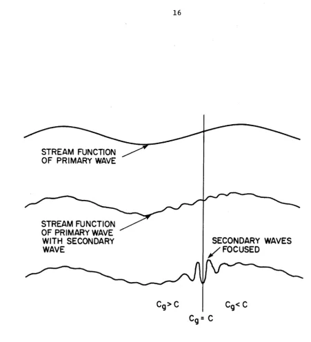
1/4 locally, although not everywhere, thus allowing the local onset of instabilities. Woods (1968, 1969) felt that this phenomenon was responsible for the observed sudden onset of turbulence in stable layers.

Landahl (1972) has given criteria for the breakdown of a flow perturbed by a wavelike disturbance of finite amplitude. The basic idea behind his theory is that the primary disturbance modifies the flow in such a way that unstable secondary waves are focused at a location where they can suddenly attain large amplitudes (see Figure 2.2.1). The following conditions apply for a two-dimensional problem. The first condition is that the group velocity, c , of the secondary

g

(48)

STREAM FUNCTION

OF PRIMARY WAVE

STREAM FUNCTION

OF PRIMARY WAVE

WITH SECONDARY

WAVE

Cg>C

SECONDARY WAVES

/FOCUSED

Cg< C

Cg= C

Figure 2.2.1 Breakdown of a flow due to focusing of a secondary disturbance.

Top: Stream function of primary disturbance to the mean flow.

Middle: Primary and secondary wave; group velocity cg of secondary wave varies along the phase of the primary wave.

[image:48.593.56.508.60.557.2]

(49)

ac fac

the primary wave itself is unstable, then the condition is c = - ____& ___£

g

at

ax

where the derivatives are taken holding the wave number constant. The second condition for focusing of the waves is that the quantity cg - c decrease through the critical point where c - c = 0. If this condition

g

holds, then waves close to the critical point will tend to move toward the critical point. For detailed discussions, see Landahl (1972) and Landahl and Criminale (1977).

The primary requirement that allows one to use Landahl's theory is that the wave number, k, of the secondary disturbance be much larger than that of the primary wave. Then, inhomogeneities in the fluid caused by the primary wave are small over one wavelength of the secondary wave. Landahl (1972) applied the theory to the sudden onset of turbulence in a boundary layer. Landahl and Criminale (1977) applied the theory to some simplified models of stratified shear flows, in particular, to flows which exhibited discontinuities in the density profile. Thorpe (1978a) considered the breaking of finite amplitude waves in a density-stratified shear flow. The photographs in his paper show properties that are

remarkably similar to properties predicted by the theory of Landahl (1972) and Landahl and Criminale (1977). In particular, a series of his photographs show large waves which begin to break with the

"appearance of thin laminae near the crest." However, shortly after this disturbance occurred on the primary wave, large amplitude

(50)

mechanism proposed by Landahl (1972), the theory and the experiment do match qualitatively, and the work by Landahl and Criminale (1977) does correctly predict the phase along the primary wave at which the break-down occurs.

Work along lines similar to those of Landahl and Criminale (1977) was done by Gartrell (1977), and the basic results are presented here.

This work was done under the supervision of M. T. Landahl in the Geophysical Fluid Dynamics program at the Woods Hole Oceanographic Institution.

The flow considered was a flow in which the density was a

con-tinuous function of depth; usually in a stability analysis disconcon-tinuous density profiles are assumed as they result in problems which are some-what more tractable. The mean flow considered is given by

and

u = 0

po =

1, y

>

1

-1, y

< -

1

A -a

y

>

1 P e

0

" -ay

poe '

!YI

~ 1

A a

y

<

-1 P e

0

(2.2.1)

(2.2.2)

(51)

y

I

II

x

uo=O

-1

m

u

0

=-I

uo=I

P

=~

e-a

0

p=~

e-ay

0

p

=$..ea

0

(52)

au + au au

_-~

x-momentum p pu - + pv - =

at ax ay ax

(2.2.3)

y-momentum p au + pu - + p v -av av =

-

~-

pg

at ax ay ay

(2.2.4)

continuity au + av = 0

ax ay

(2.2.5)

incompressibility .££_ + .££_ + ~ =

at u ax v ay 0 (2.2.6)

Equation 2.2.6 requires that the density of a fluid particle remain constant as it moves.

A

stream function is introduced such that

a'¥

u

=

u (y) + - and v

= -

~x , where '¥ is the stream function of the

o ay a

primary wave perturbation; the density is given by p

=

p

0(y) + p1(x,y,t)

where pl is the perturbation in the density. To facilitate the reduction of the equations, the transformations p

1 = p l/ 2

G and '¥ = p -l/2 ijJ are

0 0

made. Substituting the transformations into Equations 2.2.2-2.2.6, eliminating the pressure term and retaining only the first order perturbation quantities, one obtains

and

+ 1/J u (-(__.:;.__o_)

2- -

l

:>) -

_1 _a

(P

auo) 1/J - gG = O x o ₄P 2 2 P P ay o ay x x

0 0 0

Gt+ u G

0 x

(2.2.7)

(53)

where the subscripts x, y, and t denote partial derivatives. Wavelike perturbation quantities in x and t are then assumed:

1jJ = cf> (y) exp (ik(x - ct)) (2.2.9)

G = f(y) exp(ik(x- ct)) • (2.2.10)

Substituting these relations into Equations 2.2.7 and 2.2.8, one finds:

f =

o

for

I

y

I

>

1 (2.2.11)

a2 a

cf>" - cf>(k2

+ -

-

ga/ c 2 ) = 0, f = ~ for

I

y

I

~ 1 •

4

c (2.2.12)

In addition, it is required that the fluid particle displacement~

n,

be continuous across the interfaces at y = ±1 and that the pressure also be continuous. Furthermore, it is required that the perturbation quantities vanish at y = ±00 •

Three cases may be distinguished, according to whether

a2y2

=

k2

+

a2/4 - ga/c2 is equal to, less than, or greater than zero. If a2y2 is less than zero,cf>(y) is wavelike in they-direction; if a2y2

is greater than zero, cf>(y) is exponential in character. Since these two cases are similar mathematically, they will be considered together, following an analysis for y2

=

O.

Case 1, y2

=

O

Here, the solutions are:

(54)

Now n, the fluid particle displacement, is given by:

n

=

'¥I

(c - u } 0

For convenience, the solutions are written as:

'¥

1 =

o

1( c- l}exp(i0 - k(y-1) +a/2)

'¥

11 = c(Ay+B1)exp(i0+ay/2)

'¥

111

=o

111(c+l}exp(ie+k(y+l) -a/2)

n

11 = (Ay+B1)exp(i8+ay/2)

(2.2.13c)

(2.2.14)

(2.2.15a) (2.2.15b) (2.2.15c)

(2.2.16a) (2.2.16b) (2.2.16c)

where the subscripts I, II and III refer to the regions y

>

1,

I

y

I

<

1 and y

<

-1, respectively; where

e

= k(x - ct) and both

o

₁and

o

₁II are constant. The boundary conditions require

nI(l) = nII(l), nII(-1)

=

nIII(-1) and 3'¥II(l) 31J!rr(-l) o'l'II(-1)

ay ' Cc + 1) ay

=

c ay

- - - =

c

ay

where the last two equations are obtained from the Bernoulli equation. Applying the boundary conditions to (2.2.15) and (2.2.16) it is found that:

(55)

oIII =-A+ B

1 (continuity of n at y = -1) (2.2.17b)

2 a 2 . 2

(c+l) oIIIk=-z

c

(B

1-A) +c A(continuity of pressure at y=-1) (2.2.17d)

In order to obtain nontrivial solutions, i t is required that

where the facts that 2Ri = ga and y 2 = 0 have been used. This is the

dispersion relation for y2 = O.

Case 2, y 2 :f:. O

The solutions for this case are:

c1>

1 a: exp (-k(y - 1)) y > 1 (2.2.19a)

(2.2.19b)

cj>IIIa:exp (k(y + 1)) y

<

-1 (2.2.19c)

Following the same procedure as in the previous case, one finds

'l'I = (c - 1) oiexp(iS - k(y -1) + a/2) (2.2.20a)

11' = c(D eayy+D e-ayy) exp(iS+ay/2)

II 1 2 (2.2.20b)

'!'III= (c + 1) oIIIexp(ie + k(y + 1) - a/2) (2.2.20c)

(2.2.2la)

n = (D eayy+D e-ayy) exp(iS+ay/2)

(56)

(2.2.2lc)

The boundary conditions require: ay -ay

cS =De +De

I 1 2 (continuity of Tl at y = 1) (2.2.22a) (continuity of Tl at y = -1) (2.2.22b)

(continuity of (2.2.22c) pressure, y = 1)

(continuity of (2.2.22d) pressure at y = -1)

Again, for non-trivial solutions, the dispersion relation is obtained:

tanh(2ay) [c-4 (2k2 ) + 2akc3 - c2(2k2+2Ri) +k2 ] + 2ayk[c '+ +c2 ] = 0 (2.2.23)

If layl

<<

1 then Equation 2.2.23 reduces to

where the approximation tanh e:~ e: forle:I

<<

1 has been used. Equation 2.2.23 then reduces to Equation 2.2.17 when layl approaches zero.

For the case that y2 is real and negative, the amplitudes of the perturbation quantities are wavelike in the region of non-zero density gradient. Equation 2.2.22b, in this case, is of the form

D a = -D a* (2.2.25)

1 2

where the * superscript denotes the complex conjugate. This implies that ln

(57)

n

11 = b exp i8 where

e

may include an arbitrary phase and b is real, then D

1 +D2 is real (from Eq. 2.2.2lb) and, therefore, D1 =Dz*. This means that the amplitude of ~II is wavelike in the y-direction, but the waves are standing waves. Hence, waves travel only in the x-direction.

By setting y2 to zero and using Equation 2.2.18, which is the

dispersion relation for this case, curves in the wave number-Richardson number plane can be found which separate the regions for the different types of solutions. Equation 2.2.18 can be rewritten as:

c:4a.2 (c2 -1)2k2

+

kc 2 (c 2

+

2a.c

+

l}

-2- = 0 with Ri = c22 (k2

+

a.42)

Then, c can be used as a parameter to find the values of k and Ri. Two branches are found, one for c < 1 and the other for c

>

1. These are shown in Figure 2.2.3 for the case where a.= lo- 3• These curves correspond to one root of the quadratic equation for k. The other root corresponds to k< 10-6 and can be neglected for the purposes of this discussion. The regions of wavelike amplitudes of the perturbation are shown on Figure 2.2.3.

As stated previously, the conditions leading to breakdown of the flow by secondary waves are that the secondary waves be unstable and of much smaller scale than the primary wave, and that the group velocity of the secondary waves be equal to the phase velocity of the neutral primary wave. The group velocity of an unstable wave generated by shear

(58)

50

40

30

Ri

20

10

0 0

0.3

0.2

Ri

0.1

0 0

O'

Q,i;

.__-\

~~

" !=::i

::..~~

~~9.."V

.f

2 4 6 8

k

WAVELIKE

AMPLITUDES (y2<o)

0.4 0.8

k

EXPONENTIAL AMPLITUDES (y2:>D)

10 12

EXPONENTIAL AMPLITUDES(y2

>o

1.2 14