JIT Mixed Model Sequencing Rules: Is There a Best One?

(1)

http://dx.doi.org/10.4236/ajor.2015.51002

JIT Mixed-Model Sequencing Rules: Is There

a Best One?

Patrick R. McMullen

School of Business, Wake Forest University, Winston-Salem, North Carolina, USA

Email:

[email protected]

Received 3

November 2014; revised 29

November 2014; accepted 10

December 2014

Copyright © 2015 by author and Scientific Research Publishing Inc.

This work is licensed under the Creative Commons Attribution International License (CC BY).

http://creativecommons.org/licenses/by/4.0/

Abstract

This research effort compares four sequencing rules intended to smooth production scheduling

for mixed-model production systems in a Just-in-Time/Lean manufacturing environment (“JIT”

hereafter). Each rule intends to schedule mixed-model production in such a way that

manufactur-ing flexibility is optimized in terms of system utilization, units completed, average process

in-ventory, average queue length, and average waiting time. A simulation experiment, where the

various sequencing rules are tested against each other in terms of the above production measures,

shows that three of the sequencing rules essentially offer the same performance, whereas one of

them shows more variation.

Keywords

JIT/Lean Manufacturing, Scheduling, Sequencing, Enumeration, Simulation

1. Introduction

In a JIT/Lean manufacturing environment, it is important to schedule production in such a way that units are

manufactured in direct proportion to their demand. Otherwise, in-process inventories accumulate, throughput

time increases, schedule compliance suffers, all resulting in sub-optimal performance

[1]

. Consider the simple

example where four units of Item A are demanded, two units of Item B are demanded and one unit of Item C is

demanded. One possible schedule is as follows: AAAABBC. While changeovers are minimized, units are not

sequenced proportional to demand. The following schedule would be better in terms of “smoothing out”

produc-tion in terms of demand: ABACABA

[2]

.

(2)

This paper explores four of the more common sequencing rules, uses them to sequence mixed-model

produc-tion schedules, simulates producproduc-tion schedules under various condiproduc-tions, and analyzes the performance of the

various rules.

2. Sequencing Rules

Four sequencing rules are investigated for this research effort. Prior to presenting the individual rules, a few

definitions are needed.

Symbol Definition

i Index for all items

n Number of all items

(

i=1, 2,,n

)

k Index for each unique item

i

d Demand for unique item i

(

k=1, 2,,di

)

D Total number of items (or total demand)

i

∆ Average gap between units of each unique item

i k

∆ Actual gap between positions k + 1 and k for item i

ik

x The number of units of i produced through the kth_{sequence position}

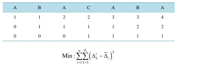
As an example for the sequence: ABACABA, we have

∆

ik

values of (2, 2, 2, 1) for

i

=

1 (Item A), (4, 3)

for

i

=

2 (Item B), and (7) for

i

=

3 (Item C). When we calculate these

∆

ik

values, we assume that the

se-quence cycles over and over. For the

∆

i

values, we simply use

D d

i

( )

∀

i

, yielding values of

(

7 4 , 7 2 , 7 1

)

for this particular problem.

2.1. Minimize Maximum Response Gap (MRG)

The first objective function to be studied is the minimization of the maximum response time for a sequence

[3]

.

Mathematically, this is as follows:

(

)

min : max max

i_k _i

i k

∆ − ∆

(1)

For our example problem, this objective function value would be as follows:

(

)

(

)

(

)

(

)

max max 2 7 4 , 2 7 4 , 2 7 4 , 1 7 4 , max 4 7 2 , 3 7 2 , max 7 7 1

−

,

which reduces to:

max 0.75, 0.50, 0.0

(

)

=

0.75 .

2.2. Minimize Average Gap Length (AGL)

The next objective to be studied is the minimization of the average distance between the actual gap and the

av-erage gap

[4] [5]

. Mathematically, this is as follows:

1 1

min :

i

d n

i k i i k

D

= =



∆ − ∆







∑∑

(2)

The example problem above, the objective function value would be as follows:

2 7 4

1 7 4

4 7 2

3 7 2

7 7 1

7  −

+ −







, resulting in a value of 0.3571.

2.3. Minimize Gap Variation (VAR)

(3)

A B A C A B A

1 1 2 2 3 3 4

0 1 1 1 1 2 2

0 0 0 1 1 1 1

(

)

2

1 1

Min :

i

d n

i k i i= k=

∆ − ∆

∑∑

(3)

Using the example problem above, the objective function value would be:

(

) (

2

) (

2

) (

2

) (

2

) (

2

) (

2

)

2

2 7 3

−

+ −

2 7 3

+ −

2 7 3

+ −

1 7 3

+ −

4 7 2

+ −

3 7 2

+ −

7 7 1

. This calculation results in a

value of 1.25.

2.4. Minimize Usage Rate (USAGE)

The final objective function to be explored is the minimization of the usage rate—keeping as constant as

possi-ble in assigning units for sequencing

[7]

. Mathematically, this is as follows:

2

1 1

Min :

i

d D

i ik k i

d

x

k

D

= =



₋











∑∑

(4)

For the example problem, the objective function value is 1.7143, when using

x

ik

values reflecting the

se-quence:

A B A C A B A

1 1 2 2 3 3 4

0 1 1 1 1 2 2

0 0 0 1 1 1 1

3. Experimentation

To determine which of the sequencing rules is most effective in terms of the JIT/Lean objectives mentioned

pre-viously, experimentation is conducted. Several problem sets are simulated according to their best sequence in

terms of the objectives described above, simulation is performed, data is collected from the simulation, and

analysis is made in an attempt to differentiate performance among the four presented objectives

[8]

.

3.1. Problem Sets

Eight problem sets are used for experimentation, starting with a small problem and having the problems grow

large to the point where finding the optimal sequencing (via complete enumeration) in terms of the objective

function values becomes computationally intractable.

Table 1

shows the product mix details of the eight

prob-lem sets used, and the number of total permutations required for compute enumeration.

Complete enumeration is used for each problem set so that the optimal values for each objective function

shown above are obtained. It is intended to show each objective function in its “best possible light”.

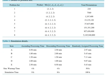
[image:3.595.167.500.81.188.2]

For each unique item, a processing time for the single-stage simulation has been assigned. In actuality, three

different processing time templates have been assigned to each unique item: ascending processing times,

de-scending processing times, and randomly assigned processing times on the uniformly-distributed interval (2, 10).

Table 2

summarizes the processing times for each of the three variants, along with simulation settings.

3.2. Simulation Outputs

Several output measures are used to determine the performance of the sequencing rules. They are as follows:

• Utilization―the average amount of time the system is busy.

• Units completed―the average number of units completed by the system.

(4)

[image:4.595.104.527.90.389.2]

Table 1.

Details of problem sets.

Problem Set Product Mix

(

d d d dA, B, C, D,dE

)

Total Permutations

1 (3, 2, 2) 210

2 (3, 2, 2, 2) 7560

3 (4, 2, 2, 2) 1,247,400

4 (5, 3, 2, 2, 2) 15,135,120

5 (6, 3, 2, 2, 2) 37,837,800

6 (6, 4, 2, 2, 2) 151,351,200

7 (6, 4, 3, 2, 2) 857,656,800

8 (6, 4, 3, 3, 2) 5,145,940,800

Table 2.

Simulation details.

Item Ascending Processing Time Descending Processing Time Randomly Assigned Processing Time

A 0.50 min 2.50 min 2.97 min

B 1.00 min 2.00 min 5.43 min

C 1.50 min 1.50 min 7.11 min

D 2.00 min 1.00 min 9.87 min

E 2.50 min 0.50 min 5.43 min

Sim. Warmup Time 4 h 4 h 50 h

Simulation Time 8 h 8 h 100 h

• Average Queue Length

―average number of units waiting to be processed.

• Average Waiting Time

―average amount of time a unit spends waiting to be processed.

These performance measures are actual outputs from the simulation.

3.3. Design of Experiment

The general research question pursued is to determine whether or not the sequencing rules have an effect on the

simulation performance measures. This question can be adequately addressed via Single-Factor ANOVA, with

the sequencing rule as the experimental factor (of which there are four levels), and the simulation-based

per-formance measure as the response variable.

Because there are eight different production models, three different processing time templates, and five

dif-ferent simulation-based performance measures, there are (8) (3) (5) = 120 difdif-ferent analyses to perform. Each of

the (120) analyses utilize (25) simulation replications.

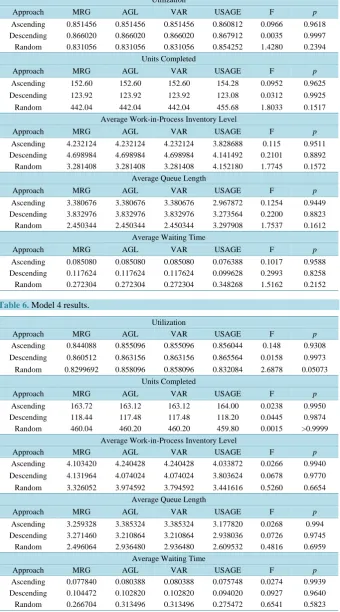
4. Experimental Results

Tables 3-10

show the results of the experiments for each unique analysis, specifically including the mean for

each factor level, along with the F-statistics and associated p-value for each experiment. These tables show that

the sequencing rule has an effect on the performance measure of interest (26) times of the (120) experiments

conducted, using an

α

=

0.05 level of significance. Of these (26) times, USAGE is a superior performer

com-pared to the other three (8) times, and is an inferior performer comcom-pared to the other three (17) times. There is

one other occasion where the sequencing rule has an effect on a performance measure of interest, but the

differ-ence is not due to USAGE.

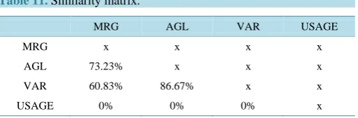
Table 11

shows the similarity between all four of the sequencing objectives, based upon the sequences

ob-tained via complete enumeration of all possible sequences for all (120) problems.

(5)

[image:5.595.143.486.109.718.2]

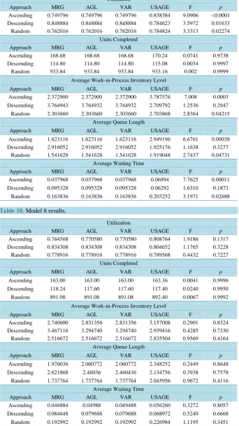
Table 3.

Model 1 results.

Utilization

Approach MRG AGL VAR USAGE F p

Ascending 0.8496 0.848500 0.846880 0.824560 1.0424 0.3764 Descending 0.8520 0.852016 0.852016 0.854600 0.0053 0.9995 Random 0.8379 0.837924 0.837924 0.833301 0.0769 0.9724

Units Completed

Ascending 217.64 195.64 217.56 216.40 10.673 <0.0001 Descending 99.16 99.19 99.16 99.76 0.0248 0.9947

Random 514.88 514.88 514.88 515.24 0.0014 >0.9999 Average Work-in-Process Inventory Level

Average Queue Length

Ascending 3.027608 2.891458 2.865168 2.581624 0.148 0.9308 Descending 2.789324 2.789324 2.789324 2.511084 0.0758 0.973

Random 2.618324 2.618324 2.618324 2.470504 0.0553 0.9828 Average Waiting Time

Table 4.

Model 2 results.

Utilization

Units Completed

Random 416.84 416.84 416.84 415.32 0.0299 0.9930 Average Work-in-Process Inventory Level

Random 3.156824 3.191032 3.191032 3.332632 0.0939 0.9633 Average Queue Length

(6)

[image:6.595.144.485.108.721.2]

Table 5.

Model 3 results.

Utilization

Units Completed

Average Work-in-Process Inventory Level

Average Waiting Time

Table 6.

Model 4 results.

Utilization

Units Completed

Ascending 163.72 163.12 163.12 164.00 0.0238 0.9950 Descending 118.44 117.48 117.48 118.20 0.0445 0.9874 Random 460.04 460.20 460.20 459.80 0.0015 >0.9999

(7)

[image:7.595.144.485.108.720.2]

Table 7.

Model 5 results.

Utilization

Random 0.877564 0.877564 0.877564 0.809252 16.531 <0.0001 Units Completed

Ascending 168.80 168.80 168.80 170.64 0.139 0.9365 Descending 114.56 114.56 114.56 114.28 0.0036 0.9997 Random 515.28 515.28 515.28 474.76 17.051 <0.0001

Random 4.646360 4.646360 4.646360 2.961892 3.0055 0.03414 Average Queue Length

Random 0.357648 0.357648 0.357648 0.222064 2.7119 0.04923

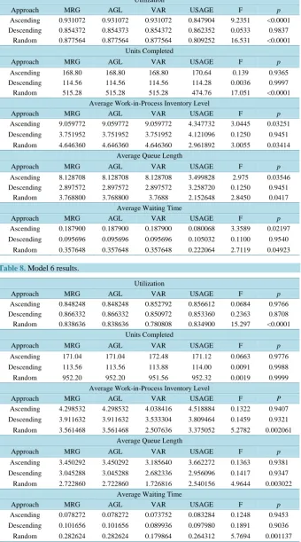
Table 8.

Model 6 results.

Utilization

Ascending 0.848248 0.848248 0.852792 0.856612 0.0684 0.9766 Descending 0.866332 0.866332 0.850972 0.853360 0.2363 0.8708 Random 0.838636 0.838636 0.780808 0.834900 15.297 <0.0001

Units Completed

Approach MRG AGL VAR USAGE F P

(8)

[image:8.595.143.486.109.719.2]

Table 9.

Model 7 results.

Utilization

Ascending 0.749796 0.749796 0.749796 0.838384 9.0906 <0.0001 Descending 0.848884 0.848884 0.848884 0.784623 3.5972 0.01633 Random 0.762016 0.762016 0.762016 0.784824 3.3313 0.02274

Units Completed