Effluent Discharges from Two Outfalls on a Sloping Beach

http://dx.doi.org/10.4236/am.2014.519295

Effluent Discharges from Two Outfalls on a

Sloping Beach

Anton Purnama

Department of Mathematics and Statistics, College of Science, Sultan Qaboos University, Muscat, Sultanate of Oman

Email: [email protected]

Received 15 August 2014; revised 10 September 2014; accepted 7 October 2014

Copyright © 2014 by author and Scientific Research Publishing Inc.

This work is licensed under the Creative Commons Attribution International License (CC BY).

http://creativecommons.org/licenses/by/4.0/

Abstract

A marine outfall is a long pipeline that continuously discharges large amounts of effluent streams into the sea. As the number of marine outfalls along the coastal areas is growing, a far field ma-thematical model with two point sources on a sloping beach is used to assess the coastal water quality following discharges from two outfalls. Asymptotic approximation will be made to the concentration at the beach to measure how well the effluent plumes are mixed and diluted in the coastal waters. The result found agrees with the engineering practice of installing a two-port dif-fuser at the end of a single outfall to minimize its potential environment impacts.

Keywords

Advection Diffusion Equation, Far Field Model, Two-Port Diffuser, Two Point Sources

1. Introduction

Most coastal industrial installations and plants, such as municipal sewage treatment plants [1] [2], power gener-ation stgener-ations [3], and seawater desalination plants [4]-[8], dispose of their wastewater effluents through long outfall pipes that stretch far into the ocean. For a modern plant, a multiport diffuser would also be installed at the pipe-end to rapidly dilute the effluent stream. Because of relatively shallow coastal waters, it is observed that the elongated effluent plumes are spreading towards the shoreline and may cause a concentration build-up [9]-[11]. Due to the uncertainty in sea conditions, a clear understanding of the mixing processes of effluent plumes is not yet known, and the use of mathematical models has been a key strategy for the basis of sound engineering de-sign and for assessing the potential environmental impacts of marine outfall effluent discharges [2] [3] [5]-[8].

effluent plumes are expected as many outfalls often tend to be closely clustered together along the coastal areas. Newly-constructed coastal plants may need to build two outfalls as a contingency plan for a future increase in the plant’s production capacity [6]. For two outfalls discharging a given integrated total effluent stream, the waste load can be allocated optimally between them to minimise the impact [12] [13].

As coastal industrial plants are built predominantly on the sloping sandy beaches, a mathematical model using a two-dimensional advection diffusion equation with two point sources is presented. The solution is plotted to graphically study the merging of two effluent plumes from two outfalls. While the far field modelling in this paper involves drastic simplifications, key physical mixing and dispersion processes are represented, and thus the analytical solution remains useful in providing a qualitative understanding and in suggesting general beha-viour of the marine outfall effluent discharge plumes in coastal environment [9] [11] [12].

2. Mathematical Analysis

The beach is considered to be straight and the sea wide, and the outfall’s effluent plume is assumed to be verti-cally well-mixed over the water depth. The coastal (drift) current is assumed to be steady with a speed U and remains in the

x

-direction parallel to the beach at all times. The dispersion mechanisms are represented by eddy diffusivities, and diffusion in the

x

-direction is neglected, as the effluent plumes in steady currents become very elongated in the

x

-direction. The variations in the y-direction of U and coefficient of dispersivity

D

are assumed as the power functions only of water depth h, and for application, we take U to be proportional to 1 2

0

h and

D

to 3 2 0

h , where h₀ is an arbitrary reference water depth. These scalings are appropriate for a turbulent shallow water flow over a smooth bed [9]-[11] [14]. For simplicity, other complexities such as tidal motions, density and temperature are ignored.

As illustrated in Figure 1, we represent the old outfall as a point source at the position

(

x₀=0,y₀=αh₀

)

discharging an effluent stream at a constant rate Q₀, where

α

is the source length. Similarly, the new outfall as a point source at

(

x₁= −h₀,y₁=

(

α ε+

)

h₀

)

discharges at a rate Q₁, where

ε

is the outfall’s (offshore) and



(along the shore) separation distances. Without loss of generality, we also assume that if these two out-falls are operated by one plant discharging, then a combined effluent total rate Q=Q₀+Q₁.

As the water depth is gradually decreasing towards the beach at y=0, on a uniformly sloping beach with slope

m

, we formulate h y

( )

=my. Following [9] [11] and applying a linear superposition, the two-dimen- sional advection-diffusion equation for the far field plume concentration c x y

(

,

)

from the two point sources is given by

(

)

0

(

0

) (

0

)

1

(

1

) (

1

)

c

hUc hD Q x x y y Q x x y y

x y y δ δ δ δ

 

∂ ₋ ∂ ∂ _{= + − + + −}

 

∂ ∂ _ ∂ _ , (1)

with boundary condition hD c y∂ ∂ =0 at the beach y=0, and the effluent concentration is assumed to be ul-timately dissolved far into the sea, c→0 as y→ ∞. δ is the Dirac delta function. In terms of dimension-less quantities

* 0

y= y h , x=x h_{* 0}, c x y

( )

, =c x y Q h U_*

(

_*, _*

)

₀2 ₀, q₀ =Q Q₀ and q₁=Q Q₁ ,

[image:2.595.225.405.590.712.2]

where Q denotes a reference discharge rate which usually adopts the value of the original discharge rate of the old outfall. By setting

0 0 0 h U D

λ = , 1 2

0

U=U y∗ and D=D y0 ∗3 2,

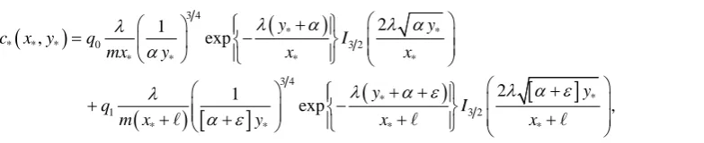
the analytical solution of Equation (1) is given by

(

)

(

)

(

)

[

]

(

)

[

]

3 4

* *

* * * 0 3 2

* * * *

3 4

* *

1 3 2

* * * * 2 1 , exp 2 1 exp , y y

c x y q I

mx y x x

y y

q I

m x y x x

λ α λ α

λ α

λ α ε

λ α ε

λ α ε   +       =   −  _ _          ₊     + +  _{ } + ₊ _{ +} _ − ₊  _{ + }       _{ }    (2)

where I_{3 2} is a modified Bessel function [15] [16]. The model parameter λ represents the effluent plume elongation in the

x

-direction [9]-[11]. In coastal waters, larger values of λ are mostly due to a stronger cur-rent U₀ with less dispersivity D₀. For the quantitative illustration of the solutions, the values of m=0.02 and λ =5 2 will be used in all plots. The other parameters are related to the position of the point sources:

α

the single point source length, and

ε

and



the point source’s separation distances.

As a higher build-up in concentration is more likely found at the shallow water close to the beach [7] [8] [10] [14], the appropriate measure for assessing the impact of marine effluent discharges from sea outfalls would be the concentration values at the beach. In the limit as y_*→0 and replacing I_{3 2} in Equation (2) by its asymp-totic form [16], we obtain the compounded concentration at the beach

(

)

5 2 5 2

(

)

* * 0 1

* * * *

4 4

, 0 exp exp

3 π 3 π

c x q q

x x x x

m m

λ α ε

λ λα λ  + 

       

≈ _{  }− _+ _{  }− _

+  + 

        . (3)

It is easy to see for effluent discharges from a single point source at

(

x₀=0,y₀=αh₀

)

and since q₀=1

(and q₁=0), the concentration at the beach reduces to

(

)

5 2

0* *

* *

4

, 0 exp

3 π c x x x m λ λα     ≈ _{  }− _    .

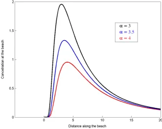
The concentration at the beach for a point source length α =3 and α=4 is plotted in Figure 2. By diffe-rentiating, the concentration has a maximum value of 5 2

0m 0.61

c ≈ mα , which occurs at the position

*m 2 5

x = λα . This maximum value is inversely proportional to the point source length

α

[9] [10]. A value of 1.96 is obtained for α =3, and this maximum value is reduced by more than 50% to 0.95 when the length is extended to α =4. This result agrees with the standard practice of building a longer sea outfall in order to mi-nimize its potential environmental impact in the coastal waters [1] [2].

3. Two Independent Outfalls

Apart from the effluent discharge rates, the compounded impact of the new outfall is governed by the outfall’s separation distances

ε

and



, and in particular, if the value of



is large (e.g. >5x_*m), the two outfalls are

well separated, and thus it is expected that the contribution of the new outfall located at

(

x₁= −h₀,

(

)

)

1 0

y = α ε+ h is negligible [9].

We first consider the case where the two outfalls are operated independently by two coastal plants, i.e., when 0 1 1

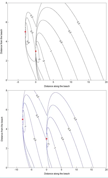
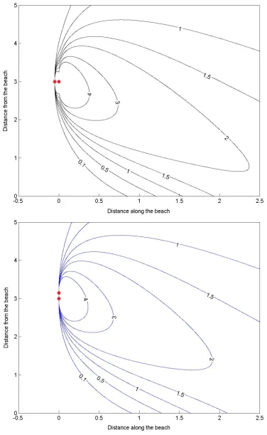
q +q ≠ and when both separation distances >0 and ε >0. The concentration contour plots of Equation (2), the solution for two point sources when α=3 and ε=2, is shown in Figure 3, which illustrates the merging of plumes from the two point sources for two values of the separation distance =3 with q₀=1 and

1 0.5

q = , and =8 with q₀=0.5 and q₁=1, where two separate plumes are clearly shown.

Since the value λ =5 2 is used in the plot, x_*m =2λα 5= =α 3 and the top part of Figure 3 represents a

situation where two outfalls are relatively close to each other at a small distance apart, = =3 x_*m, and the new

point source is discharging with a rate q₁=0.5, half of the old point source at

(

x₀=0,y₀=αh₀

)

. The bottom part of Figure 3 represents two outfalls at a slightly longer distance apart, = ≈8 2.67x_*m, where the new point

source is discharging with a rate q₁=1, double that of the old point source.

[image:3.595.132.524.116.196.2]

Figure 2.The concentration at the beach for a single point source.

(

)

(

)

* 5 2 *

* * 0* * 0 1

* * *

, 0 , 0 x exp x

c x c x q q

x x x

ε α λ  _{    − }   ≈ +  ₊  −  ₊          

[image:4.595.145.477.89.352.2]

  . (4)

Figure 4 shows the concentration at the beach for the two cases illustrated inFigure 3, where two separated plumes are depicted as two distinctive peaks. For comparison, the concentration for the single point source with

0 1

q = is also shown in Figure 4 by the dotted line. It is worth noting that for x_*>0, the presence of the new outfall does not change the location of the maximum concentration at the beach [11].

Substituting x_*m =2λα 5 in Equation (4), the maximum value of concentration at the beach for two point

sources is approximated as

( )

1m 0m 0 1 c ≈c _q +q f z _,

where z= x_*m=

(

5 2λ

)(

α

)

and

( ) (

)

5 2 5

1 exp

2 1

z

f z z

z ε α

−   − 

= + − _{ +} _

 .

By differentiating, f z

( )

has a maximum value of fm

(

1 ε α

)

5 2

−

= + , which occurs at z_m =ε α, and there-fore

5 2

1m 0m 0 1 1

c c q q ε

α −  _{ }  ≤  + _ + _     

 . (5)

[image:5.595.140.489.84.659.2]

Figure 3.Merging contour of two point sources plumes when α =3 and ε =2.

[image:6.595.145.481.84.359.2]

Figure 4.Compounded concentration at the beach for two point sources.

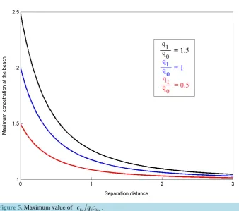
Figure 5.Maximum value of c_1m q c_{0 0m}.

4. Single Outfall with Two Ports

[image:6.595.145.484.375.674.2]

outfall lengths. For the case where two outfalls is operated by one plant, i.e. when q₀+q₁=1, the effluent dis-charge allocation can be arranged between these two outfalls [12]. Binomial expansion of Equation (5) for

1

ε α < , gives

5 2

1 0 0 1 0 1

5 7

1 1 1

2 4

m m m

c c q q ε c q ε ε

α α α

−  _{ }  _{    } ≈  + _ + _ ≈ _ − _ _{ } − + __      .

That is, the maximum value of c_1m is smaller than that of the single point source value c_0m. This result agrees with the previous finding [12] [13], that if two outfalls are discharging a given integrated total effluent stream, the waste load can be allocated optimally between them to minimise the impact. However, economically it is cheaper to build an outfall and install a two-port diffuser at its pipe-end than build one more sea outfall.

To include the case of the modern engineering practice that installs two ports at the end of a marine outfall [5] [6], we also assume that both port separation distances ε α and  α are small, and thus the value of f z

( )

can be approximated for z≤0.05 by f₀ ≈exp

(

−5ε α2

)

.

For plotting the contours of the effluent plume, since the point sources are close to each other, and in the limit as x_*→0 and replacing I_{3 2} in Equation (2) by its asymptotic form [16], we obtain

(

)

(

)

₍

₎

₍

₎

(

)

2 2 * * 0 1 * * * * * * * * *

, exp exp

4π 4π

y y

q q

c x y

m y x x m y x x

λ α λ α ε

λ λ

α α ε

 ₋   _{− +}      = _− _+ _− _ + + +           .

The contours of the solution for a single outfall with two ports are reproduced graphically in Figure 6 for 3

α= with q₀ =q₁=0.5, when z=0.05, which is equivalent to the port separation distance  α =0.05 for

5 2

λ = . The effluent plumes from these two closely located point sources are immediately merged as they are released, and for x_*>0, and the combined plumes appears to be spreading as one. This supports the concept that a two-port diffuser will rapidly dilute effluent streams.

Finally, the maximum value of compounded concentration at the beach for two closely located point sources can be approximated to

1 0 0 1 0 1

5 5 5

exp 1 1

2 2 4

m m m

c c q q ε c q ε ε

α α α

       

≈ _ + _− _≈ _ − _{ } − + _

     

    .

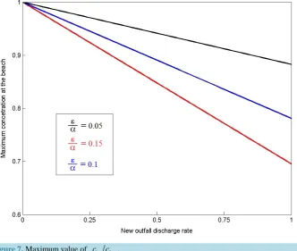
Again, the maximum value of c_1m is smaller than that of the single point source value c_0m. From Figure 7, we noted that as the value of q₁ increases and the port separation distance ε α gets longer, the maximum value becomes smaller than c_0m. For example, if ε α =0.1 and both ports are discharging at equal rates, i.e.

1 0 0.5

q =q = , then the maximum value of c_1m is about 10% less than c_0m. This result agrees with the modern engineering practice that installing a two-port diffuser at the end of a marine outfall will improve the mixing and dilution of effluent discharge plumes in coastal waters [5] [6] [12].

5. Conclusions

The solutions for an advection diffusion equation with two point sources are applied to study the interaction and merging of effluent discharge plumes from two outfalls on a sloping beach. As a measure for assessing the im-pact in the coastal environment, the maximum compounded concentration at the beach is formulated. If the two outfalls are independently operated, then the maximum value of the concentration at the beach can be minimized as long as the new outfall length is more than double the old outfall length, and discharging at a rate smaller than the old outfall.

If two outfalls are operated by one plant, then the integrated total effluent load can be shared between them, and it is found that the maximum value of the concentration at the beach is smaller than that of the single outfall. A similar result is also obtained for a single outfall where a two-port diffuser is installed at the end outfall pipe. However, implementation issues related to the control of discharge rates, reliability and cost effectiveness of the marine outfall are not addressed.

[image:8.595.125.502.85.697.2]

[image:9.595.149.482.91.372.2]

Figure 7.Maximum value of c1m c0m.

Acknowledgements

The author is grateful to Sultan Qaboos University for an Internal Grant IG/SCI/DOMS/14/01 which provided financial support for this work.

References

[1] Institution of Civil Engineers (2001) Long Sea Outfalls. Thomas Telford Ltd., London.

[2] Signell, R.P.,Jenter, H.L. and Blumberg A.F. (2000)Predicting the Physical Effects of Relocating Boston’s Sewage Outfall. Estuarine, Coastal and Shelf Sciences, 50, 59-71. http://dx.doi.org/10.1006/ecss.1999.0532

[3] Macqueen, J.F. and Preston, R.W. (1983) Cooling Water Discharges into a Sea with a Sloping Bed. Water Research, 17, 389-395. http://dx.doi.org/10.1016/0043-1354(83)90134-3

[4] Lattemann, S. and Hopner, T. (2008) Environmental Impact and Impact Assessment of Seawater Desalination. Desali-nation, 220, 1-15. http://dx.doi.org/10.1016/j.desal.2007.03.009

[5] Bleninger, T. and Jirka, G.H. (2008) Modelling and Environmentally Sound Management of Brine Discharges from Desalination Plants. Desalination, 221, 585-597. http://dx.doi.org/10.1016/j.desal.2007.02.059

[6] Purnama, A., Al-Barwani, H.H., Bleninger, T. and Doneker, R.L. (2011) CORMIX Simulations of Brine Discharges from Barka Plants, Oman. Desalination and Water Treatment, 32, 329-338. http://dx.doi.org/10.5004/dwt.2011.2718 [7] Roberts, D.A., Johnston, E.L. and Knott, N.A. (2010) Impacts of Desalination Plant Discharges on the Marine

Envi-ronment: A Critical Review of Published Studies. Water Research, 44, 5117-5128. http://dx.doi.org/10.1016/j.watres.2010.04.036

[8] Palomar, P. and Losada, I.J. (2011) Impacts of Brine Discharge on the Marine Environment. Modelling as a Predictive Tool. In: Schorr, M., Ed., Desalination, Trends and Technologies, InTech Open Access Publisher, Rijeka, Croatia, 279-310.

[9] Al-Barwani, H.H. and Purnama, A. (2009) Analytical Solutions for Brine Discharge Plumes on a Sloping Beach. De-salination and Water Treatment, 11, 2-6. http://dx.doi.org/10.5004/dwt.2009.835

[11] Purnama, A. (2012) Merging Effluent Discharge Plumes from Multiport Diffusers on a Sloping Beach. Applied Ma-thematics, 3, 24-29. http://dx.doi.org/10.4236/am.2012.31004

[12] Smith, R. and Purnama, A. (1999) Two Outfalls in an Estuary: Optimal Wasteload Allocation. Journal of Engineering Mathematics, 35, 273-283. http://dx.doi.org/10.1023/A:1004332007489

[13] Bikangaga, J.H. and Nassehi, V. (1995) Application of Computer Modeling Techniques to the Determination of Opti-mum Effluent Discharge Policies in Tidal Water Systems. Water Research, 29, 2367-2375.

http://dx.doi.org/10.1016/0043-1354(95)00045-M

[14] Smith, R. (1976) Longitudinal Dispersion of Buoyant Contaminant in a Shallow Channel. Journal of Fluid Mechanics, 78, 677-688. http://dx.doi.org/10.1017/S0022112076002681

[15] Murphy, G.M. (1960) Ordinary Differential Equations and Their Solutions. D. Van Nostrand, London.