HYBRID OPTIMIZATION FOR GRID SCHEDULING USING GENETIC ALGORITHM WITH LOCAL SEARCH

HYBRID GREEDY – PARTICLE SWARM OPTIMIZATION –

GENETIC ALGORITHM AND ITS CONVERGENCE TO

SOLVE MULTIDIMENSIONAL KNAPSACK PROBLEM 0-1

1_{FIDIA DENY TISNA A.,} 2_{SOBRI ABUSINI,} 3_{ARI ANDARI} 1

P.G. Student, Department of Mathematics, Brawijaya University, Indonesia

2,3

Lecturer, Department of Mathematics, Brawijaya University, Indonesia

E-mail: [email protected], [email protected],[email protected].

ABSTRACT

In this research, we present a hybrid algorithm called Greedy – Particle Swarm Optimization – Genetic Algorithm (GPSOGA). This algorithm is based on greedy process, particle swarm optimization, and some genetic operators. Greedy algorithm is used as initial population, Particle Swarm Optimization (PSO) as main algorithm and Genetic Algorithm (GA) as support algorithm. Multidimensional knapsack problem 0-1 (MKP 0-1) will be used as test problem. To solve MKP 0-1, GPSOGA divided into 3 variants: GPSOGA (1), GPSOGA (2), and GPSOGA (3) based on criteria how they choose an initial solution in each algorithm. Then we will see which variant that is better to solve MKP 0-1, in term of the best solution ever known, the

average of solution in each run, and the average of computational time. After 20×running program

individually, we can see that GPSOGA (3) is more suitable than GPSOGA (1) and GPSOGA (2) to solve MKP 0-1. Because it can solve the test problem more accurate, and have better average solution except in Data 2 and Data 3. We also provide convergence analysis to GPSOGA solution. So, it can be proved that GPSOGA solution is always convergent to global optimum and it can’t exceed the exact solution in solving MKP 0-1.

Keywords: Genetic Algorithm, Greedy Algorithm, Multidimensional Knapsack Problem 0-1, Particle

Swarm Optimization.

1.

INTRODUCTION

In 2011, Singh et al [1] introduced binary particle swarm optimization with crossover operation to solve discrete optimization function. He combines the binary particle swarm optimization and genetic crossover operator to improve the solution diversity. Five different types of binary crossover operators are used to binary particle swarm optimization to check whether the hybrid algorithm works better on benchmark function or not. The result shows that proposed algorithm give better results for few standard benchmark functions.

Greedy algorithm is a simple and fast algorithm because it only chooses solution which is described in greedy criteria. Many paper used greedy as combination to their hybrid algorithm in the hope the greedy solution can help the hybrid algorithm to close to the nearest solution. Mizan et al [2] used greedy method to find the nearest cloud storage center and recourses in a hybrid cloud. Pramanik et

al [3] present new hybrid classifier that combines

the k-Nearest Neighbor (k-NN) and ID3 algorithm. In [3], greedy algorithm is used to constructs

decision trees in a top-down recursive divide and conquer manner. Labey and Chence [4] used greedy in the first phase to create a feasible solution for bin packing problem in their algorithm, called Greedy Randomized Adaptive Search Procedure (GRASP).

The multidimensional knapsack problem 0-1 is known as NP-Hard problem [5]. Some research [6-8] had solved this problem well. But most of them didn’t provide convergence analysis for MKP 0-1 solution that has been obtained.

In this paper, we propose a hybrid algorithm called Greedy-PSO-Genetic Algorithm (GPSOGA) based on greedy algorithm and binary PSO with crossover operation. We used a different crossover technique and add mutation operator to increase the

diversity probability. The multidimensional

convergence analysis to guarantee that GPSOGA solution is convergent to solve MKP 0-1. It is required to see the behavior of GPSOGA solutions.

2.

GENERAL MODEL OF MULTIDIMENSIONAL KNAPSACK PROBLEM 0-1, GREEDY ALGORITHM, GENETIC ALGORITHM, AND PARTICLE SWARM OPTIMIZATION.

2.1 Multidimensional Knapsack Problem 0-1

The multidimensional knapsack problem 0-1 is an optimization problem. It can be described as given a set of items that have two attributes, profit and weights, and a knapsack with some constraints. Our objective is to maximize the sum of profit by choosing items without exceeding the knapsack constraints. Mathematically, it can be formulated as follows [9]:

Maximize

∑

= n

i 1

pixi , i=1,…,n (E1)

Subject to

∑∑

= = m

j n

i

1 1

wijxi≤Wj, (E2)

xi∈{0,1}, j=1,…m

Where pi is the profit of i-th item, xi is the criteria

of choosing an item (1, if the item is chosen and 0,

otherwise), wij is the weight of the i-th item and j-th

constraint, Wj is the maximum capacity of

knapsack/constraints, m is the number of

constraints, n is the number of items.

2.2 Greedy Algorithm

Greedy algorithm will take one of feasible solutions in each turn and add it to the previous solution. In the hope, the last solution will converge to global optimum. There are 3 methods in greedy algorithm to solve KP 0-1 [10]:

(1) choose item with the highest profit (p>>)

(2) choose item with the lowest weight (w>>)

(3) choose item with the highest ratio (p/w>>)

2.3 Genetic Algorithm

Genetic Algorithms were invented by John Holland. Holland developed Genetic Algorithms with his students and colleagues. This lead to Holland's book "Adaption in Natural and Artificial Systems" published in 1975 [11]. GA is inspired by genetic process in human body and there are four

processes in this algorithm: population, selection, crossover, and mutation.

2.4 Particle Swarm Optimization

Particle Swarm Optimization was introduced by Eberheart and Kennedy in 1995 [12]. PSO is inspired by social behavior of bird flocking, animal hording, or fish schooling to search food in an area [5]. The potential solutions are called particle. Each particle will move depend on its velocity and the two best positions known (its own and that of the swarm) according to the following two equations:

vikt+1=w.vikt+c1.r1t.(pbikt-xikt)+c2.r2t.(gbt-xikt) (E3)

xik

t+1

=xik

t

+vik

t+1

(E4)

w is an inertia coefficient. (xikt+1, xikt), (vikt+1, vikt):

position and velocity of particle k in dimension i at

times t+1 and t, respectively. pbikt, gbt: the best

position obtained by the particle k and the best position obtained by the swarm in dimension i at

time t, respectively. c1, c2: two constants

representing the acceleration coefficients [13]. r1t,

r2

t

: random numbers drawn from the interval [0,1] at time t.

3.

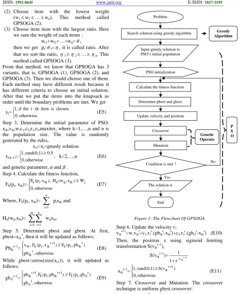
BASIC IDEA OF GPSOGA

Every algorithm has strength and weakness. With the description in previous section, we know that greedy algorithm is a fast algorithm but sometimes the greedy solution only approach the global solution. PSO is an algorithm that based on the best particle in its population. Because in PSO, the other particles in the population converge towards the best particle’s position. The better particle’s position, the faster PSO solves a problem. Genetic operators, like crossover and mutation are used to vary the solution. So, we put greedy solution to PSO initial population in the hope it can make PSO population better. Then add some genetic operators (crossover and mutation) in the hope it can find solution which is too far away from PSO population. The flowchart of GPSOGA can be seen at Figure 1.

4.

APPLICATION OF GPSOGA FOR MKP 0-1

The step of GPSOGA to solve MKP 0-1 can be described as follows:

Step 1. Input the problem. Input pi, wij, and Wj.

Step 2. Search the problem solution using greedy algorithm. There are 3 methods to get the solution:

(1) Choose item with the highest profit

(p1≥p2≥…≥pn). This method called

(2) Choose item with the lowest weight

(w1≤w2≤…≤wn). This method called

GPSOGA (2).

(3) Choose item item with the largest ratio. Here

we sum the weight of each items :

wi1+wi2+…+wij=θi

then we get pi/θi=η, it is called ratio. After

that we sort the ratio, η1≥ η2≥…≥ηn. This

method called GPSOGA (3).

From that method, we know that GPSOGA has 3 variants, that is, GPSOGA (1), GPSOGA (2), and GPSOGA (3). Then we should choose one of them. Each method may have different result because it has different criteria to choose an initial solution. After that we put the items into the knapsack as order until the boundary problems are met. We get

xi=

   otherwise. 0, chosen is item th -i the if 1, (E5)

Step 3. Determine the initial parameter of PSO:

xik,vik,w,c1,c2,r1,r2,maxiter, where k=1,…,u and u is

the population size. The value is randomly generated by the rules,

xi1=xi=greedy solution

xi(k-1)=

   _≥ otherwise 0, 0.5 rand(0,1) 1,

, k=2,…,u (E6)

and genetic parameter,αandβ.

Step 4. Calculate the fitness function,

Fk(pi, xik)=

    _≤ otherwise 0, W ) x , (w H ), x , (p

F_{k i ik k ij ik j}

(E7)

Where, Fk(pi, xik)=

∑

= n

i 1

pixik and

Hk(wij,xik)=

∑∑

= = m j n i 1 1

wijxik.

Step 5. Determine pbest and gbest. At first,

pbest=xik1, then it will be updated as follows:

Pbikt+1=

    + _≥ otherwise. , pb ) pb , (p F ) x , (p F , x ik t ik i k 1 t ik i k ik t (E8)

While gbest=zeros(size(xi1)), it will updated as

follows:

gbi1t+1=

[image:3.612.85.554.77.652.2]

    + + _≥ otherwise , gb ) gb , (p F ) pb , (p F , pb t i1 t i1 i k 1 t ik i k 1 t ik (E9)

Figure 1: The Flowchart Of GPSOGA

Step 6. Update the velocity v,

vikt+1=w.vikt+c1.r1t.(pbikt-xikt)+c2.r2t.(gbi1t-xikt) (E10)

Then, the position x using sigmoid limiting

transformation S(vikt+1),

S(vik

t+1

)= _{t 1}

ik v -e 1 1 + +

xikt+1=

    _≥ + otherwise. 0, ) S(v rand(0,1)

1, ikt 1 _(E11)

Step 7. Crossover and Mutation. The crossover technique is uniform gbest crossover:

xikt+1=

    + _≤ otherwise. rand(0,1) , gb , x t i1 1 t

ik α _(E12)

Where α is the crossover rate. The value of α is

between 0-100%.

Search solution using greedy algorithm Problem

Input greedy solution to PSO’s initial population

Yes

No PSO initialization

Condition is met ? Calculate the fitness function

End The solution is

gbest

Determine pbest and gbest

Update velocity and position

Then the mutation process is

xikt+1=

  

 _≤

+ +

otherwise. ,

x

rand(0,1) , x

1 t ik

1 t

ik β _(E13)

Where xikt+1 is the binary invers of xikt+1 and β is

the probability of mutation process happen.

Step 8. Repeat step 4-7 until maxiter condition is satisfied. The global solution of GPSOGA is gbest in the last iteration.

5.

EXPERIMENTAL RESULT

[image:4.612.94.296.292.401.2] [image:4.612.100.291.449.509.2]

The data test is taken from ORLib [14]. The data test is called mknap1.txt which can be seen from Table 1.

Table 1: The Data Test.

Data

Test Items Constraints

Exact Solution

Data 1 6 10 3800

Data 2 10 10 8706.1 Data 3 15 10 4015

Data 4 20 10 6120

Data 5 28 10 12400

Data 6 39 5 10618

Data 7 50 5 16537

The parameter can be seen from Table 2.

Table 2: The Parameter Of Algorithms.

Algorithm Parameter

PSOGA c1=c2=2 inertia value (w)=1 crossover rate (α)=0.333

mutation rate (β)=0.05 GPSOGA (1)

GPSOGA (2) GPSOGA (3)

We used population size=30 and maximum iteration (maxiter)=100 to save computational time. Then we will compare each type of GPSOGA and PSOGA which is can be described as GPSOGA without greedy algorithm, in term of, the best solution ever known, the average of solution in each run, and the average of computational time.

After 20×running program individually using

Matlab, running on Core2Duo 2.0GHz and 2GB of RAM, we get

Table 3: The Best Solution Ever Known.

Algorithm

Data PSOGA

GPSOGA

(1) (2) (3) Data 1 3800 3800 3800 3800

Data 2 8706.1 8706.1 8706.1 8706.1

Data 3 4015 4015 4015 4015

Data 4 6120 6120 6120 6120

Data 5 12400 12390 12400 12400

Data 6 10559 10537 10584 10588 Data 7 16440 16374 16405 16456

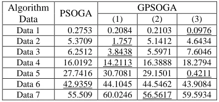
Table 3 shows the best solution ever known. In other words, it can be used to measure the accuracy of algorithm. The bigger value of the solution, the closer it to exact number. The bold printed values show that the algorithm succeed to get the exact number and the underlined values show that they can’t get the exact solution, but they are the best value ever obtained compared to others. It can be seen that GPSOGA (3) get the best solution ever known bigger than GPSOGA (1), GPSOGA (2), and PSOGA in Data 6 and Data 7.

Table 4: The Average Solution In Each Run.

Algorithm

Data PSOGA

GPSOGA

(1) (2) (3) Data 1 3800 3800 3800 3800

Data 2 8537.2 8706.1 8540 8558.4 Data 3 4013.5 4014.5 4010.5 4011 Data 4 6069.5 6087.5 6104.5 6105 Data 5 12307 12282 12308 12400

Data 6 10453 10317 10433 10459 Data 7 16147 16145 16164 16282

Table 4 shows the average solution in each run

after 20×running program. It can be seen that

GPSOGA (3) get the average solution better than the others in Data 4, Data 5, Data 6, and Data 7 and GPSOGA (1) get the better solution in Data 2 and Data 3. It means, GPSOGA (3) solutions close to exact solution than the others in each run in Data 4, Data 5, Data 6, and Data 7 and GPSOGA (1) solutions close to exact solution in Data 2 and Data 3.

Table 5: The Average Computational Time In Each Run.

Algorithm

Data PSOGA

GPSOGA

[image:4.612.307.528.626.729.2]

Table 5 shows the average computational time in each run (in seconds). It can be seen that GPSOGA (1) can solve faster in Data 2, Data 3, and Data 4. Although, the difference between algorithms are less than 5 seconds except in Data 5. In Data 5, GPSOGA (3) can solve faster because it get exact solution in its initial population. In other words, the greedy solution get the exact solution in GPSOGA (3) initial population. This is what we hope from the hybrid algorithm.

6.

THE CONVERGENCE OF GPSOGA TO SOLVE MKP 0-1

The convergence of GPSOGA can be seen from the series of its solution in each iteration. Numerically, it can’t be guaranteed that the solution will stop at any value. Therefore, we need an analytic process to guarantee that the solution will stop at certain value. Some of real analysis definition [15] will be used to guarantee that the GPSOGA solution is convergent.

DEFINITION 6.1

Let S ⊂ℜ , S said

(a) Bounded above, if ∃α∈ℜ ∋x≤α,∀x∈S.

ub={α∈ℜ|x≤α,∀x∈S} is called upper

bound S, if UB is an upper bound of S but no number less than UB is, then UB is a supremum of S , and we write UB = Sup S.

(b) Bounded below, if ∃β∈ℜ ∋x≥β ,∀x∈S.

lb={β∈ℜ|x≥β ,∀x∈S} is called lower

bound S, if LB is a lower bound of S but no number greater than LB is, then LB is a infimum of S , and we write LB = Inf S

(c) Bounded, if a nonempty set has a unique

supremum and a unique infimum, and

LB≤UB.

DEFINITION 6.2

Let D ⊂ℜ so that D contain interval I and

f:D→ℜis a function, then f said

(1) Nondecreasing on I if x1,x2∈I, x1<x2

⇒f(x₁)≤f(x₂) and

(2) Nonincreasing on I if x1,x2∈I, x1<x2

⇒f(x₁)≥f(x₂).

“The series of GPSOGA solution in solving MKP 0-1 are convergent if the sequence of GPSOGA fitness function is nondecreasing and bounded“

Let M is called the maximum profit of knapsack

without worrying the constraints. So, M=

∑

p

where p is the set of profit on each item. Now, we ignore the index i because it has no effect on this proof, but one of the most influential is the index k because it shows a different individual. From Step 4, the fitness value of MKP 0-1 can be rewritten as

f(xk)=

     

≤

∑

∑

=

otherwise. 0,

W x w , px

m

1 j

j k j k

(E14)

Where xk = the k-th solution, k=1,…,u

wj = the j-th weight set

Wj = the j-th constraint

∑

= m

j 1

wjxk≤Wj is the sum of j-th weight multiplied

by the k-th solution less than equal to the j-th

constraint. For each k=1,…,u, we have

P={f(x1),f(x2),…,f(xu)}. P is called set of fitness

function. Because M is the maximum profit of knapsack problem, then we can conclude that

f(xk)≤M,∀k=1,…,u. It means, if

smax=argmax(f(xk)|k=1,…,u), we also say that smax

is the maximum solution of population in one

iteration, f(smax)≤M. Any real number is greater

than equal to f(smax) is upper bound of P. f(smax) is

upper bound of P but no number less than f(smax) on

upper bound of P, then f(smax) is a supremum of P

………(P1)

For the lower bound, assume that there are no item

selected or xk={0}, then the profit is

m=

∑

pxk=

∑

p.0=0 (minimum profit). From

Equation (E14), for each k=1,…,u, we have

P={f(x1),f(x2),…,f(xu)}. Because m is the minimum

profit of knapsack problem, then we can conclude

that m≤f(xk),∀k=1,…,u. It means, if

smin=argmin(f(xk)|k=1,…,u), we also say that smin is

the minimum solution of population in one

iteration, m≤f(smin). Any real number is less than

equal to f(smin) is lower bound of P. f(smin) is lower

bound of P but no number greater than f(smin) on

lower bound of P, then f(smin) is a infimum of P

………(P2)

and infimum in one iteration and it is the same for each iteration. So, we can say the fitness function of GPSOGA solutions is bounded in each iteration and it is kept in interval [0,M] by Equation (E14). Although the infimum and supremum may be different in each iteration ………(P3)

Next, we will see the solution of GPSOGA in one run. Here, we are focused on the maximum solution

(smax) in each iteration. From (P3), we can conclude

smax∈[0,M]. If S={s1,s2,…,smaxiter} is the set of

GPSOGA solution in each iteration, where st=smaxt

(it is called the maximum solution of GPSOGA in

t-th iteration), then st∈[0,M], ∀t=1,…,maxiter.

Corresponding to gbest in Step 5, it can be rewritten as

st+1=

 

 _{+ + ≥}

otherwise. ,

s

) f(s ) f(s , s

t

t 1 t 1 t

(E15)

Where st = gbi1t = the solution of t-th iteration and

f(st) = F(pi,gbi1t) =

∑

p.st = the fitness value of

t-th iteration, t=1,…,maxiter. Consequently by (E15),

for each s1,s2,…,smaxiter∈S, index 1<2<…<maxiter

⇒f(s₁)≤f(s₂)≤…≤f(s_maxiter). It means that the

sequence of fitness function is nondecreasing on S …………(P4)

From (P4) we know that f(s1) is the minimum

number of S and f(smaxiter) is the maximum number

of S. By using some variables in (P1) and (P2), we can write again,

1) m≤ f(s1). Any real number is less than equal

to f(s1) is lower bound of S. f(s1) is lower

bound of S but no number greater than f(s1)

on lower bound of S, then f(s1) is a infimum

of S.

2) f(smaxiter)≤M. Any real number is greater than

equal to f(smaxiter) is upper bound of S.

f(smaxiter) is upper bound of S but no number

less than f(smaxiter) on upper bound of S, then

f(smaxiter) is a supremum of S.

3) S has supremum and infimum, then S is

bounded ………(P5)

From (P4) and (P5) we can conclude that the series of fitness function S are nondecreasing and bounded..

Here is, the illustration of GPSOGA convergence theory by solving MKP 0-1 test data with GPSOGA

(3) in 1× running program. And it will be the same

with the other GPSOGA, the difference is the fitness values in each iteration.

0 10 20 30 40 50 60 70 80 90 100 3799

3799.2 3799.4 3799.6 3799.8 3800 3800.2 3800.4 3800.6 3800.8 3801

P

ro

fit

o

r

F

it

n

e

s

s

V

a

lu

e

Iteration

Figure 2: The Result of GPSOGA (3) for DATA 1

0 10 20 30 40 50 60 70 80 90 100 8300

8350 8400 8450 8500 8550 8600 8650 8700 8750

P

ro

fit

o

r

F

it

n

e

s

s

V

a

lu

e

Iteration

Figure 3: The Result of GPSOGA (3) for DATA 2

0 10 20 30 40 50 60 70 80 90 100 3820

3840 3860 3880 3900 3920 3940 3960 3980 4000 4020

P

ro

fit

o

r

F

it

n

e

s

s

V

a

lu

e

[image:6.612.314.514.58.599.2]

Iteration

0 10 20 30 40 50 60 70 80 90 100 6010

6020 6030 6040 6050 6060 6070 6080 6090 6100 6110

P

ro

fit

o

r

F

it

n

e

s

s

V

a

lu

e

Iteration

Figure 5: The Result of GPSOGA (3) for DATA 4

0 10 20 30 40 50 60 70 80 90 100 1.2399

1.2399 1.2399 1.24 1.24 1.24 1.24 1.24 1.2401 1.2401 1.2401x 10

4

P

ro

fit

o

r

F

it

n

e

s

s

V

a

lu

e

[image:7.612.87.527.68.610.2]

Iteration

Figure 6: The Result of GPSOGA (3) for DATA 5

0 10 20 30 40 50 60 70 80 90 100 0.98

0.99 1 1.01 1.02 1.03 1.04 1.05 1.06x 10

4

P

ro

fit

o

r

F

it

n

e

s

s

V

a

lu

e

[image:7.612.100.283.446.595.2]

Iteration

Figure 7: The Result of GPSOGA (3) for DATA 6

0 10 20 30 40 50 60 70 80 90 100 1.58

1.59 1.6 1.61 1.62 1.63 1.64x 10

4

P

ro

fit

o

r

F

it

n

e

s

s

V

a

lu

e

Iteration

Figure 8: The Result of GPSOGA (3) for DATA 7

7.

CONCLUSION

In this paper, we present a hybrid algorithm called GPSOGA. To solve MKP 0-1, GPSOGA is divided into 3 variants: GPSOGA (1), GPSOGA (2), and GPSOGA (3). The experiment shows that GPSOGA (3) can get more accurate result in term of the best solution ever known than GPSOGA (1), GPSOGA (2), and PSOGA. In term of the average of solution in each run, GPSOGA (1) has better results in Data 2 and Data 3, then GPSOGA (3) has better results in Data 4, Data 5, Data 6, and Data 7. And the solution of GPSOGA in solving MKP 0-1 is guaranteed convergent.

Though, we say the proposed algorithm is used to solve small MKP 0-1. Hence, further comparison is needed in a large problem. Compared to other algorithm in past 5 years, this algorithm is still lack of accuracy. It needs to find another greedy criteria so it can get the initial solution better and simplify PSO and GA process so it can save computational time. The last, the convergence analysis is only applied to solve MKP 0-1. So, the global convergence of GPSOGA needs to provide.

REFRENCES:

[1] Singh, Deepak., Singh, Vikas., and Ansari, Uzma., “Binary Particle Swarm Optimization with Crossover Operation For Discrete

Optimization”, International Journal of

Computer Applications (Vol. 28 No. 11),

August, 2011, pp. 15-20.

[2] Mizan, Tasquia., Al Masud, Shah Murtaza Rasyid., And Latip, Rohaya., “Modified Bee

Life Algorithm for Job Scheduling”,

International Journal of Engineering and Technology (Vol. 2 No. 6), June, 2012, pp.

[3] Pramanik, Shovon K., Pramanik, Subrata., Pramanik, Bimal K., Molla, M.K Islam., and Hamid, Md. Ekramul., “Hybrid Classification Algorithm for Knowledge Acquisition of Biomedical Data”, International Journal of

Advanced Science and Technology (Vol. 44),

July, 2012, pp. 99-112.

[4] Layeb, Abdesslem., and Chence, Sara., “A Novel GRASP Algorithm for Solving the Bin

Packing Problem”, I.J. Information

Engineering and Electronic Business, 2012,

pp. 8-14.

[5] Abdelhalim, M.B., and Habib, S.E., “Particle

Swarm Optimization for HW/SW

Partitioning”, Particle Swarm Optimization, In-Tech Publisher, 2009, pp. 49-76.

[6] Ling, Wang., Xiuting, Wang., Jingqi, Fuu., and Lanlan, Zen., “A Novel Probability Binary Particle Swarm Optimization Algorithm and Its Application”, Journal Of Software (Vol. 3 No. 9), December, 2008, pp. 28-35.

[7] Zhibao, Mian., “Meta-heuristics for

Multidimensional Knapsack Problems”,

IPCSIT (Vol. 39), 2012.

[8] Deane, Jason., and Agarwal, Anurag., “Neural, Genetic, And Neurogenetic Approaches For Solving The 0-1 Multidimensional Knapsack

Problem”, International Journal of

Management & Information Systems (Vol. 17

No. 1), 2013, pp. 43-54.

[9] Varnamkhasti, M. Jalali., “Overview of the Algorithms for Solving the Multidimensional Knapsack Problems”, Advanced Studies in

Biology (Vol. 4 No. 1), 2012, pp. 37-47.

[10] Hristakeva, Maya., and Dipti Shresta.,

“Different Approach to Solve The 0-1 Knapsack Problem”, Midwest Instruction and

Computing Symposium, 2005.

[11] Khurana, Narnita., Rathi, Anju., and P.S, Akshatha., “Genetic Algorithm: A Search of Complex Spaces”, International Journal of

Engineering and Technology (Vol. 2 No. 6),

June, 2012, pp. 13-17.

[12] Dorigo, M., “Particle Swarm Optimization”,

www.schoolarpedia.com, revision #52052, 2008.

[13] Labed, Said., Gherboudj, Amira., and Chiki, Salim., “A Modified Hybrid Particle Swarm Optimization For Solving The Traveling Salesman Problem”, Journal of Theoretical

and Applied Information Technology (Vol. 39

No. 3), 15 May 2012, pp. 132-138.

[14] http://people.brunel.ac.uk/~mastjjb/jeb/orlib/

files/mknap1.txt.

[15] Trench, Willian F., “Introduction To Real Analysis”, Library of Congress