DESIGN, ANALYSIS AND OPTIMIZATION OF A MICROSTRIP PATCH ANTENNA AT FREQUENCY 3 55 GHZ FOR WIMAX APPLICATION

THE MISSILE TARGET EXTRACTION IN ULTRAVIOLET

IMAGES WITH NOISE AND BURST INTERFERENCES

1,2

GAO QINA, 1,2ZHU YIING, 2ZOU PING

1

The school of Electronic and Information Engineering 2

Beijing University of Aeronautics and Astronautics, Beijing 100191, China

E-mail: [email protected]

ABSTRACT

Though ultraviolet warning systems are working at sun-blind wave-band, while this paper reveals that in the ultraviolet (UV) images of the systems for missile approaching, there exist strong noise and burst interferences coming from UV CCD electronic sensors and high gain amplifiers. The CCD interferences can not be effectively removed by classical 2-D filtering algorithms, while they will influence the detection of the missile target in the ultraviolet images. To solve the problem, unchanging the current hardware structure of UV CCD electronic sensors, this paper develops a 3-D filtering algorithm for imaging sequence based on a 3-D recursive filter, which is stable and it extracts the missile target clearly. The proposed 3-D recursive filter composes of a 2-D spatial-filtering IIR and 1-D time-filtering IIR, both are stable. The stability test algorithms are provided. The proposed 3-D recursive filter is of much less computation amount UV image sequences and it can realize fast and real-time image filtering. Simulation experiments of UV image processing have shown that the proposed 3-D filtering and related algorithms are correct effective and pragmatica1.

Key words: Ultraviolet Image; Burst Interference; 3D Recursive Filtering; Missile Target Extraction

1. INTRODUCTION

Many astronomical objects produce orders of magnitudes more photon fluxes at optical wavelengths than they do in the vacuum UV. In order to eliminate this huge background contribution and substantial source of noise solar-blind detector and imaging systems are required [1-6]. Conventional high-end imaging applications utilize large format full-frame and frame transfer style CCD image sensors. The benefits of using this architecture are high sensitivity, high charge capacity and low dark currents resulting in very large dynamic ranges. These CCDs are typically front-side illuminated and tend to have lower sensitivity or Quantum Efficiency (QE) for wavelengths less than 500nm (UV). The UV sensor can be applied for discovering and following the missile plume at solar-blind wave-band and it can give warning to missile.

Because most of the ultraviolet radiations of the sun are absorbed by the ozone layer in the earth atmosphere, part of the ultraviolet spectral range is blank. Consequently, when a missile is jetting ultraviolet radiations it can be probed easily by

ultraviolet photo-detecting system. This property has been utilized widely in the military area, especially ultraviolet warning technology. We use MODTRAN 4 get the atmospheric transmittance at the solar-blind wave-band, 250nm-280nm (UV), shown in Fig.1. This band will be used to detect the missile plume. MODTRAN (MODerate spectral resolution atmospheric TRANsmission) is a Fortran based atmospheric transmission model and has been established as the standard for simulating a number of scenarios especially within imaging and signals and sensor performance [7]. The MODTRAN Code calculates atmospheric transmittance and radiance for frequencies from 0 to 50,000 cm-1 at moderate spectral resolution (Every 2 cm-1 or 20 cm-1 in UV range). Effects

taken into consideration include spherical

refractive geometry, solar and lunar source functions, and scattering (Rayleigh, Mie, single and multiple).

uncertain burst interferences or noise coming from a UV CCD electronic sensor, where neither the sun nor missile is in the UV imaging window.

0.250 0.255 0.26 0.265 0.27 0.275 0.28 1

2 3 4 5 6x 10

-3

WAVELENGTH/MICRONS

T

O

T

A

L

T

R

A

N

[image:2.612.108.278.143.283.2]

S

Figure 1: The atmospheric transmittance at the solar-blind wave-band: 250nm-280nm (UV)

Figure 2: The interferences or noise coming from a UV CCD electronic sensor

A pre-warning system of a fighter working at the UV wavebands can recognize jetting ultraviolet radiations when the enemy missile is approaching to the fighter. This is very important to gain time for fighter’s reaction. We expect that the UV solar-blind spectral band is utilized to obtain the image of target and scene clearly and in detail. However, the detecting capability for missile with lower UV radiation are weaken by the random burst interferences or UV CCD imaging noise on the UV imaging system, there exist the interferences or noise coming from UV CCD electronic sensors and high gain amplifiers.

From Fig. 2 we can see that it is not easy to extract missile target from the random interferences or noise if signal amplitude of missile target is nearly to those of the interferences or noise. Generally, the random interferences or noise in Fig.2 arc difficult to be canceled by exiting 2-D spatial filtering algorithms [8-14], including Lee filter, Kuan filter,

Sigma filter and Frost filter. The main problem of the existing 2-D filtering algorithms is that time-direction filtering has not been considered. To solve the problem, this paper extends the 2-D leapfrog digital filter [15] to 3-D IIR digital filter to remove the noise and interference. The proposed 3-D IIR digital filter is a stable 3-D recursive digital filter with nearly linear phase that avoids the image phase distorting, and it is stable, it can realize the fast filtering for UV image sequences.

The 2-D hybrid transforms (DFT-DWT and DCT-DWT) in [13, 14] for image denoising, involve huge calculation for their wavelet transform, DFT and DCT, it is hard to realized fast or real-time 2-D filtering so that extending them to 3-D has no meaning. The further problem is the computation amount of 3-D filtering [17-21]. It is not practical to use 3-FIR filters, which generally need buffer 100 UV frames to get good filtering quality. While, the 3-D IIR (recursive) filters may suffer the stability problems [22-25].

The above problems can be solved by the proposed 3-D recursive filter, which only buffers two processed UV frames for recursive filtering without stability problem. This paper provides the design and difference equations’ implementation algorithms of 3-D IIR digital filter. Simulations for UV images verify the proposed 3-D recursive filter, show that the proposed 3-D recursive filtering can extract the missile objects from strong noise and interference.

2. PROBLEM FORMULATION

Ultraviolet (UV) rays are an invisible form of light which lie slightly beyond the violet end of the visible spectrum. The sun is the major natural source of ultraviolet rays. Lightning and other electrical sparks in the air also emit ultraviolet rays. The UV rays can also be produced artificially by passing an electric current through a gas or vapor, such as mercury vapor. UV rays have shorter wavelengths than visible light. A wavelength, defined as the distance between the crests of two waves, is often measured in units called nanometers (nm) for UV description. A nanometer is a billionth of a meter, or about 1/25,000,000inch. UV wavelengths are sometimes quoted in Angstrom-an Angstrom is a unit length

equal to 10-10 meters. Typically UV wavelengths

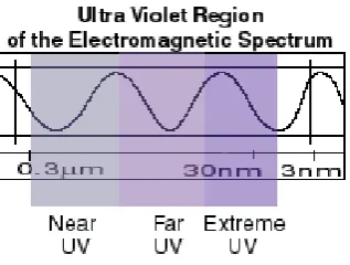
[image:2.612.118.289.333.454.2]

[image:3.612.120.279.358.478.2]

As shown in Fig. 3, the ultraviolet bandwidth of the electromagnetic spectrum is divided into three regions: the Near Ultraviolet (NUV), the Far Ultraviolet (FUV), and the Extreme Ultraviolet (EUV). The regions are sometimes designated as A, B, and C. The three regions are distinguished by the energy level of the ultraviolet radiation and the "wavelength" of the ultraviolet light, which is related to energy. The NUV region is closest to optical or visible light band. EUV is closest to X-rays and is the most energetic of the three types. The FUV region lies between the near and extreme ultraviolet regions. The flames of missiles have the characteristics of UV light, and they are of the wavelength of 220nm~280nm in the "solar blind wave-band". The solar blind UV Intensifier Charge Couple Devise (ICCD) can detect the missiles and realize imaging. Because the UV targets be detected are weak signals mostly, need to use amplifiers to intense them, the weak target signal and noise are inevitably amplified.

Figure 3:The ultraviolet bandwidth of the electromagnetic spectrum

In the solar blind wave-band, the UV images detected by UV CCD have the following characteristics.

1) The burst interferences in spatial domain occupy the high frequency part of the spatial frequency domain. In time domain, The burst interferences are temporal and un-continuous. 2) The missile objectives are continuous in both spatial domain and time domain.

3) There is no obvious spatial structure or frequency structure of the noise of the imaging sequence in spatial domain or frequency domain, and the noise occupy high-frequency part at the time direction of the imaging sequence.

4) The image noises or interferences come from the photocathode dark electronics emission and photoelectron noise of the optical detection device and the main image intensifier.

5) The random noises or interferences locate in different locations in the image, and their intensity may be large or equal to the strength of missile goals, and similar with missile objectives with the low frequency components of the UV image.

We can see from the above analysis, to effectively extract the goals from the UV image sequence, we should mainly reduce the image noises or the interferences, while the characteristics (1) and (2) remind us that the proposed 3-D IIR should be a 3-D low-pass filter.

Now, we define the 3-D discrete imaging sequence to be

y n n n

( ,

_{1 2}

,

₃

)

,

x n n n

( ,

_{1 2}

,

₃

)

to be the desired object,

w n n n

( ,

_{1 2}

,

₃

)

to be the random noises or interferences,

n

₁,

n

₂and

n

₃ are horizontal variable, vertical variable, and time variable of the image

sequence, respectively, where

0

≤ ≤

n

₁

N

₁ ,

2 2

0

≤

n

≤

N

and

0

≤

n

₃

≤

N

₃ .

N

₁ ,

N

₂

and

N

₃are the lengths of the 3-D sequence along

three directions. In this paper, to solve the problem of fast filtering, we will limit

N

1

=

N

2

=

N

3

=

2

for the proposed 3-D IIR filter, which means we only need buffer 2 frames for 3-D filtering.

We establish the signal model for the imaging sequence

y n n n

( ,

_{1 2}

,

₃

)

with noise or burst interferences as following,

1 2 3 1 2 3 1 2 3

( , , ) ( , , ) ( , , )

y n n n =x n n n +w n n n (1)

For the CCD output

y n n n

( ,

_{1 2}

,

₃

)

, the intensity of

1 2 3

( ,

,

)

w n n n

may be large or equal to the strength of

x n n n

( ,

_{1 2}

,

₃

)

, which will lead to a wrong warning for missile approaching.

This paper proposes following 3-D IIR digital filter to remove the noise term

w n n n

( ,

_{1 2}

,

₃

)

, H z z z( ,_{1 2}, ₃)=H z z H zs( ,_{1 2}) t( )₃ (2) where

H z z

_s

( ,

_{1 2}

)

is a 2-D IIR digital filter, which completes the spatial filtering along x and y directions, and

H z

t

( )

3 is a 1-D IIR digital filter,

1 2 1 2 1 2 1 2 1 2 1 2

1 2 1 2 0 0

1 2

1 2 1 2 0 0

( ,

)

( ,

)

( ,

)

K K k k s k k

s K K

k k

s k k

a k k z

z

H z z

b k k z

z

− −

= =

− −

= =

=

∑ ∑

∑ ∑

(3)

3 3 3 3 3 3 3 3 0 ₃ 3 3 3 3 0

( )

( )

( )

( )

( )

K k t k _t t K k t t k

a k z

A z

H z

B z

b k z

−

=

−

=

=

∑

=

∑

(4)

From (3) and (4), we can get the following 2-D IIR filtering algorithm and 1-D IIR filtering algorithm.

1 2

1 2

1 2

1 2 1 2

1 2 3

1 3 1 1 2 2 3

0 0

1 2 1 1 2 2 3

0 0,( , ) (0,0)

( , , ) ( , ) ( , , ) ( , ) ( , , ) K K s k k K K s k k k k

z n n n

a k k y n k n k n

b k k y n k n k n

= = = = ≠ = − − − − −

∑ ∑

∑

∑

(5) and 3 3 3 3

1 2 3 3 1 2 3 3

0

3 1 2 3 3

1 ( , , ) ( ) ( , , ) ( ) ( , , ) K t k K t k

u n n n a k z n n n k

b k u n n n k

= = = − − −

∑

∑

(6)

Equations (5) and (6) are the two filtering equations of the proposed 3-D IIR digital filter.

Equations (5) and (6) are recursive difference equations. The stability of them will be tested following Theorem 1. We can see from (5) and (6), the number of multiplications for one pixel much few, and there is no DFT and IDFT calculations. Thus, it is possible for 3-D IIR filter to realize fast and real-time filtering.

Here, the problem to be solved is to design a stable 3-D IIR digital filter. We can obtain the characteristic polynomials of the 2-D IIR filter (3) and the 1-D IIR filter (4) as following,

1 2

1 2 1 2

1 2 1 2 1 2

0 0

( ,

)

( ,

)

K K k k s s k k

B z z

b k k z

−

z

−

= =

=

∑ ∑

(7)

3

3 3

3 3 3

0

( )

( )

K k t t k

B z

b k z

−

=

=

∑

(8)

We have following stability theorem to the proposed 3-D IIR filter.

Theorem 1: If the 3-D IIR digital filter in (2) has no non-singularities, then the 3-D IIR filter is stable if and only if

B z z

_s

( ,

_{1 2}

)

≠

0,|

z

₁

| 1,|

≥

z

₂

| 1

≥

(9) and

B z

_t

( )

₃

≠

0,|

z

₃

| 1

≥

(10) where

B z z

_s

( ,

_{1 2}

)

is given in (4).

The proof can be obtained by referring [22-25]. The stability condition of

B z

_t

( )

₃ in (6) is easy, many well known tool can be found. While, to test the stability condition of

B z z

s

( ,

1 2

)

in (5)

is some difficult. To solve the problem, we provide following theorem [22-25].

Theorem 2: If the 2-D polynomial

B z z

_s

( ,

_{1 2}

)

is stable if and only if

B z

_s

( ,1)

₁

≠

0,|

z

₁

| 1

≥

(11) and

j 1

2 1 2

(e

,

)

0,

,|

| 1

s

B

ω

z

≠

ω

∈

R z

≥

(12)

There are two problems to apply the 3-D IIR filter in (2): one is stability problem, we had to design the 3-D IIR filter satisfy the conditions of Theorem 1; the other is that the designed 3-D IIR filter need to remove the noise term

w n n n

( ,

_{1 2}

,

₃

)

.

3. DESIGN OF STABLE 3-D IIR FILTER

From (2), we need to design stable

1 2

( ,

)

s

H z z

and

H z

_t

( )

₃ . The design of

H z

_t

( )

₃

is easy, we can refer [15] and obtain a low-pass filter,

1 2

,0 ,1 3 ,2 3 3

3 1 2

,1 1 ,2 3 3

( ) ( )

1 ( )

t t t t

t

t t t

a a z a z A z

H z

b z b z B z

− −

− −

+ +

= =

+ + (13)

where

2 2

,0 , , ,

,1 ,0

,2 ,0

3

/(1 3

3

)

2

t t c t c t c

t t

t t

a

a

a

a

a

ω

ω

ω

=

+

+

=

=

(14)

2 2

,1 , , , ,

2 2

,2 , , , ,

(6

2) /(1 3

3

)

(1 3

3

) /(1 3

3

)

t t c t c t c

t t c t c t c t c

b

b

ω

ω

ω

ω

ω

ω

ω

=

−

+

+

= −

+

+

+

(15)

where

ω

t c_,

=

2

π

f

t c_,

/

f

t s_, is the cut-off angular frequency of the 1-D IIR,

f

t s, is the sampling

Since [15] established the relationship of filter

parameters and

ω

_{t c,} , we can adjust the filter

parameters according to

ω

_{t c,} . We select

ω

_{t c,} by considering the noise characteristics of UV image sequence along time axis. We design

H z

t

( )

3 as

low-pass filter since the noises or the interferences of the imaging sequence

y n n n

( ,

_{1 2}

,

₃

)

are high frequency signals.

To guarantee the designed

H z

_t

( )

₃ to be stable, we have following theorem from [25].

Theorem 3: For

b

_t,1 and

b

_t,2 given in (14), the

B z

_t

( )

₃ in (12) is stable if and only if

|1

+

b

_t,2

|

>

b

_t,1 (16)

The design of stable

H z z

_s

( ,

_{1 2}

)

is some

complicated, we derive the parameter matrices

a k k

s

( ,

1 2

)

and

b k k

s

( ,

1 2

)

by following

algorithms. Let

,0 ,1 ,2

,

1, 2

i

a

i

a

i

a

i

i

a

=



_



_

=

(17)

where

2 2

,0 , , ,

,1 ,0

,2 ,0

3

/(1 3

3

),

1, 2

2

i i c i c i c

i i

i i

a

i

a

a

a

a

ω

ω

ω

=

+

+

=

=

=

(18)

and

,0 ,1 ,2

,

1, 2

i

b

i

b

i

b

i

i

b

=



_



_

=

(19)

2 2

,1 , , ,

2 2

,2 , , , ,

(6

2) /(1 3

3

),

1, 2

(1 3

3

) /(1 3

3

)

i i c i c i c

i i c i c i c i c

b

i

b

ω

ω

ω

ω

ω

ω

ω

=

−

+

+

=

= −

+

+

+

(20) where

ω

_{i c,}

=

2

π

f

_{i c,}

/

f

_{i s,}

,

i

=

1, 2

are the cut-off angular frequencies of 2-D IIR,

f

_{i s,}

,

i

=

1, 2

are the sampling frequencies along horizontal and vertical directions, which can be different in the two directions.

Then, from (17) and (19) we obtain

1 2

(0, 0)

(0,1)

(0, 2)

(1,1)

(1,1)

(1, 2)

(2, 0)

(2,1)

(2, 2)

s s s

T

s s s s

s s s

a

a

a

a

a

a

a

a

a

A

a a









=

_{= }

_









(21) 1 2

(0, 0)

(0,1)

(0, 2)

(1,1)

(1,1)

(1, 2)

(2, 0)

(2,1)

(2, 2)

s s s

T

s s s s

s s s

b

b

b

b

b

b

b

b

b

B

b b









=

_{= }

_









(22) We can get the 2-D polynomials in

H z z

_s

( ,

_{1 2}

)

,

1 2

1 2

1 2

1 2 1

1 1 2

2 2 2 2

1 2 1 2 0 0

( , )

(0, 0) (0,1) (0, 2) 1

1 (1, 0) (1,1) (1, 2)

(2, 0) (2,1) (2, 2)

( , )

s

s s s

s s s

s s s

k k s

k k

A z z

a a a

z z a a a z

a a a z

a k k z z

− − − − − − = =           =               =

∑ ∑

(23) and 1 2 1 2 1 2

1 2 1

1 1 2

2 2 2 2

1 2 1 2 0 0

( , )

(0, 0) (0,1) (0, 2) 1

1 (1, 0) (1,1) (1, 2)

(2, 0) (2,1) (2, 2)

( , )

s

s s s

s s s

s s s

k k s

k k B z z

b b b

z z b b b z

b b b z

b k k z z

− − − − − − = =           =               =

∑ ∑

(24) According to Theorem 2, we need keep

1

( ,1)

s

B z

and j 1

2

(e

,

)

s

B

ω

z

to be stable,

1 1 2 1 2 1 1 2 2

1 2 1 0 0

( ,1)

(0, 0) (0,1) (0, 2) 1

1 (1, 0) (1,1) (1, 2) 1

(2, 0) (2,1) (2, 2) 1

( , )

s

s s s

s s s

s s s

k s

k k

B z

b b b

z z b b b

b b b

b k k z−

= =           =               =

∑ ∑

(25) and

1 1 1

1 1 2 1 2

j -j -j2

2 1 2 2 2 2 2 -j

1 2 2

0 0

(e

,

)

1 e

e

(0, 0)

(0,1)

(0, 2)

1

(1, 0)

(1,1)

(1, 2)

(2, 0)

(2,1)

(2, 2)

( ,

)e

s

s s s

s s s

s s s

k k s

k k

B

z

b

b

b

b

b

b

z

b

b

b

z

b k k

z

ω ω ω

ω − − − = =





= 





 





 



⋅

_

_{ }

⋅

_



 





 



=

∑ ∑

(26)

Theorem 4: Let

1

1

2

1 1 1

0

( ,1)

( )

k

s s

k

B z

b k z

−

=

=

∑

(27)

where

2

2

1 1 2

0

( )

( ,

)

s s

k

b k

b k k

=

=

∑

(28)

then the

B z

s

( ,1)

1 in (24) is stable if and only if

|1

+

b

s

(2) | |

>

b

s

(1) |

(29)

Similarly, j 1

2

(e

,

)

s

B

ω

z

in (26) can be regarded as

a 1-D polynomial with complex coefficients, we have following stability test theorem.

Theorem 5: Let

1 1 2

2

2

j -j

2 2 2

0

(e

,

)

(e

,

)

k

s s

k

B

ω

z

b

ω

k z

−

=

=

∑

(30)

where

1 1 1

1

2

j -jk

2 1 2

0

(e

,

)

( ,

)e

s s

k

b

ω

k

b k k

ω

=

=

∑

(31)

then j 1

2

(e

,

)

s

B

ω

z

in (25) is stable if and only if

1 1 1

j j j

|

b

s

(e

, 0)

b

s

(e

, 2) |

|

b

s

(e

,1) | 0

ω

₊

ω

₋

ω

_>

(32) where

1 1 1

1

2

j -jk

1 0

(e

, 0)

( , 0)e

s s

k

b

ω

b k

ω

=

=

∑

(33)

1 1 1

1

2

j -jk

1 0

(e

,1)

( ,1)e

s s

k

b

ω

b k

ω

=

=

∑

(34)

1 1 1

1

2

j -jk

1 0

(e

, 2)

( , 2)e

s s

k

b

ω

b k

ω

=

=

∑

(35)

Limited by the paper size, we could not provided the proof, and the proof can be obtained by referring [22-25].

4. SIMULATIONS

First, we design the proposed 3-D IIR filter that composes of

H z

_t

( )

₃ and

H z z

_s

( ,

_{1 2}

)

.

We design

H z

_t

( )

₃ by using (12)-(14), and

selecting

f

_{t c,}

=

0.2

in

ω

_{t c,}

=

2

π

f

_{t c,}

/

f

_{t s,} . Substitute

ω

_{t c,} into (13) and (14), we can obtain

the parameters

a

_t,0

=

0.1323

，

a

_t,1

=

0.2645

,2

0.1323

t

a

=

and

b

_t,1

=

-0.6289

b_t,2=0.1580. Applying Theorem 3, we can find

|1

+

b

_t,2

| |

>

b

_t,1

|

Thus

H z

_t

( )

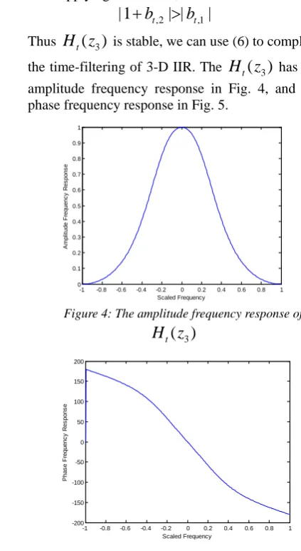
₃ is stable, we can use (6) to complete the time-filtering of 3-D IIR. The

H z

_t

( )

₃ has the amplitude frequency response in Fig. 4, and the phase frequency response in Fig. 5.

-1 -0.8 -0.6 -0.4 -0.2 0 0.2 0.4 0.6 0.8 1 0

0.1 0.2 0.3 0.4 0.5 0.6 0.7 0.8 0.9 1

Scaled Frequency

A

m

pl

it

ude F

requenc

y

R

es

pons

[image:6.612.84.523.77.539.2]

e

Figure 4:The amplitude frequency response of

3

( )

t

H z

-1 -0.8 -0.6 -0.4 -0.2 0 0.2 0.4 0.6 0.8 1 -200

-150 -100 -50 0 50 100 150 200

Scaled Frequency

P

has

e F

requenc

y

R

es

pons

e

Figure 5: The phase frequency response of

H z

_t

( )

₃

From Fig.5 we can see that the proposed IIR has linear phase property in the scaled frequency pass-band of [-0.2 0.2] Hz, which is desired for image filtering.

We design

H z z

_s

( ,

_{1 2}

)

by using (17)-(26), and selecting

f

_{i c,}

=

0.1,

f

_{i s,}

=

4

,

i

=

1, 2

in

,

2

,

/

,

i c

f

i c

f

i s

ω

=

π

. Substitute

ω

_{t c,} into (16-19),

we can obtain the parameters

,0 ,1 ,2

,

1, 2

i

a

i

a

i

a

i

i

a

=



_



_

=

where

,0

0.0889,

,1

0.1778,

,2

0.0889,

=1,2

i i i

a

a

a

i

=

=

=

[image:6.612.297.509.123.510.2]

,0 ,1 ,2

,

1, 2

i

b

i

b

i

b

i

i

b

=



_



_

=

where

,1

0.8898,

,2

0.2454, =1,2

i i

b

= −

b

=

i

.

Substitute

a

_iand

b

_iinto (21) and (22), we can

obtain

(0, 0) (0,1) (0, 2)

(1, 0) (1,1) (1, 2)

(2, 0) (2,1) (2, 2)

0.0079 0.0158 0.0079

0.0158 0.0316 0.0158

0.0079 0.0158 0.0079

s s s

s s s s

s s s

a a a

a a a

a a a

A

 

 

=  

 

 

 

 

=  

 

 

(35)

and

(0, 0) (0,1) (0, 2) (1, 0) (1,1) (1, 2) (2, 0) (2,1) (2, 2) 1 -0.8898 0.2454 -0.8898 0.7917 -0.2183

0.2454 -0.2183 0.0602 s s s s s s s s s s

b b b

b b b

b b b

B

 

 

=  

 

 

 

 

=  

 

 

(36)

From (36) and (26), we can obtain

1 1 1

j -j -j2

(0, 0)

(e

, 0)

1 e

e

(1, 0)

(2, 0)

s

s s

s

b

b

b

b

ω ω ω













=

_

_{ }

⋅

_









(37)

1 1 1

j -j -j2

(0,1)

(e ,1) 1 e e (1,1)

(2,1)

s

s s

s

b

b b

b

ω ω ω

 

 

 

=_{  }⋅ _

 

 

(38)

and

1 1 1

j -j -j2

(0, 2)

(e , 2) 1 e e (1, 2)

(2, 2)

s

s s

s

b

b b

b

ω ω ω

 

 

 

=_{  }⋅ _

 

 

(39)

Applying Theorem 5, we can find

1 1 1

j j j

|

b

s

(e

, 0)

b

s

(e

, 2) |

|

b

s

(e

,1) | 0

ω

₊

ω

₋

ω

_>

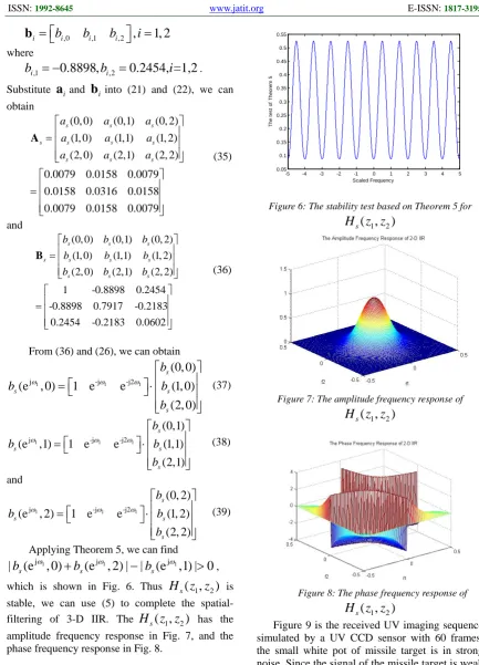
, which is shown in Fig. 6. Thus

H z z

s

( ,

1 2

)

is

stable, we can use (5) to complete the

spatial-filtering of 3-D IIR. The

H z z

_s

( ,

_{1 2}

)

has the

amplitude frequency response in Fig. 7, and the phase frequency response in Fig. 8.

-5 -4 -3 -2 -1 0 1 2 3 4 5

0.05 0.1 0.15 0.2 0.25 0.3 0.35 0.4 0.45 0.5 0.55

Scaled Frequency

T

he t

es

t of

T

heor

em

[image:7.612.84.518.74.676.2]

5

Figure 6: The stability test based on Theorem 5 for

1 2

( ,

)

s

H z z

Figure 7: The amplitude frequency response of

1 2

( ,

)

s

H z z

Figure 8: The phase frequency response of

1 2

( ,

)

s

H z z

[image:8.612.125.266.158.294.2] [image:8.612.131.247.327.455.2]

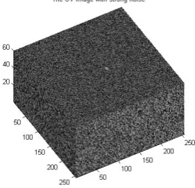
the missile target, and obtain a filtered UV imaging sequence. The last frame of the filtered UV imaging sequence is shown in Fig. 11. From Fig. 11, we can see that the proposed 3-D IIR can extract the missile target from strong noise.

Figure 9: The received UV imaging sequence

Figure 10: The last frame of the received UV imaging sequence

Figure 11: The last frame of the filtered UV imaging sequence

5. CONCLUSIONS

This paper proposed a 3-D IIR for extracting missile targets in UV images from strong noise and burst interferences. The detailed design of a stable 3-D IIR is provided. Considering that the burst

interferences in spatial domain occupy the high frequency part of the spatial frequency domain, and in time domain, the burst interferences are temporal and un-continuous; the missile objectives are continuous in both spatial domain and time domain, the proposed 3-D recursive filter adopts a 2-D spatial-filtering IIR and 1-D time-filtering IIR, which can separate the missile targets from strong noise and burst interferences. Both proposed 1-D and 2-D filters are stable, the stability test algorithms for them are provided. The stability of 1-D time-filtering IIR and 2-D spatial-filtering IIR can be tested by Theorem 3 and Theorem 5, respectively. Application of 3-D filtering for UV images is simple and valid for extracting missile targets.

REFERENCES

[1] M. Clampin, “UV-Optical CCDs”, Proceedings

of the space astrophysics detectors and detector technologies conference held at the STScI. Baltimore, June 26–29, 2000.

[2] O. H. W. Siegmund, B.Welsh, “Narrow-band tunable filters for use in the FUV region.”

Proceedings of the Space Astrophysics Detectors and Detector Technologies Conference held at the STScI. Baltimore, June 26–29, 2000.

[3] C. Joseph, “UV Technology Overview,”

Proceedings of the space astrophysics detectors and detector technologies conference held at the STSc I. Baltimore, June 26–29, 2000.

[4] M. P. Ulmer, W B.W.essels, B. Han, J. Gregie, A. Tremsin, O. H. W. Siegmund, “Advances in wide-bandgap semiconductor base photocathode devices for low light level

applications”, Proc. SPIE 5164, 144–154,

2003.

[5] O. H. W. Siegmund, “MCP imaging detector

technologies for UV instruments”, in

proceedings of the space astrophysics detectors and detector technologies conference held at the STScI. Baltimore, June 26–29, 2000.

[6] E. Wilkinson, “Maturing and developing technologies for the next generation of UV gratings ultraviolet-optical space astronomy

beyond HST”. Conference held at the STScI,

[7] A. Berk, G.P. Anderson, P. K. Acharya, J. H. Chetwynd , L.S. Bernstein, E.P. Shettle, M.W.

Matthew , and S. M. Adler-Golden,

“MODTRAN4 USER’S MANUAL”, Air

Force Research Laboratory, June 1, 1999. [8] Kazuo Ouchi, Hai peng Wang, “Interlook

Cross-Correlation Function of Speckle in SAR Images of Sea Surface Processed With

Partially Overlapped Subapertures”, IEEE

Trans on Geoscience and Remote Sensing,

Vol.43, No.4, pp.695-701, April 2005.

[9] Alin Achim, Panagiotis Tsakalides, Anastasios Bezerianos, “SAR Image Denoising via Bayesian Wavelet Shrinkage Based on

Heavy-Tailed Modeling”, IEEE Trans on Geoscience

and Remote Sensing, Vol.41,No.8, pp.1773-1784, August 2003.

[10] Juho Vihonen, Timo Ala-Kleemola, Ari Visa Elina Helander, Jani Tikkinen, “New Detection Algorithm for Poor Signal-to-Noise

Conditions”, IEEE Radar Conference, 2003,

pp.345-349.

[11] Dong-hui Hu, Yi-rong Wu, “The Scatter-Wave

Jamming to SAR”, ACTA Electronica Sinica,

Vol.30, No.12, pp.1882-1884, Dec. 2002. [12] Hua Xie, Leland E. Pierce, Fawwaz T. Ulaby,

“SAR Speckle Reduction Using Wavelet Denoising and Markov Random Field

Modeling”, IEEE Trans on Geoscience and

Remote Sensing, Vol.40, No.10, pp.2196-2212, October 2002.

[13] Y. Xiao, Y. K.Zhang, “An Approach of Extracting Object of SAR Based 2-D Hybrid

Transform”, China’s State Intellectual

Property Office, Patent Application No. 20091023-7860.6, 2009.

[14] Y. Xiao, Y. K. Zhang, “A Pre-Processing Approach for SAR Echo Denoising Based 2-D

Hybrid Transform”, China’s State Intellectual

Property Office, Patent Application No.2009100083345.7, 2009.

[15] Y. Xiao, X. Y. Du, “Realization of 2-D

Leapfrog Digital Filters”, China 1991

International Conference on Circuits and Systems, Shenzhen, June 1991, pp.609-612. [16] Y. Xiao, “Design of three-dimensional (3-D)

QMF recursive digital filter banks for HDTV”,

Proceedings of 1993 IEEE Region 10 Conference on Computer, Communication, Control and Power Engineering, (TENCON '93), 1993 , vol.3: 434-437.

[17] Sekiguchi T., Takahashi S., Matsuda K., “Design of three-dimensional spherically symmetric IIR digital filters with real and

complex coefficients using spectral

transformations”, European Conference on

Circuit Theory and Design, 1989, Page(s): 467– 471.

[18] Kuenzle B., Bruton L.T., “3-D IIR filtering using decimated DFT-polyphase filter bank

structures”, IEEE Transactions on Circuits and

Systems I, 2006, 53(2): 394–408.

[19] G.A. Boulter, J.F. Lampropoulos, “Filtering of moving targets using SBIR sequential frames”,

IEEE Transactions on Aerospace and Electronic Systems, 1995, 31(4): 1255 – 1267. [20] Djebali, M.; Melkemi, M.; Vandorpe, D.; “3-D range images segmentation based on Deriche's

optimum filters”, Proceedings of IEEE

International Conference on Image Processing, (ICIP-94), 1994 , Vol.3: 503- 507.

[21] Ip H.M.D., Drakakis E.M., Bharath A.A., “Synthesis of Nonseparable 3-D Spatiotemporal Bandpass Filters on Analog

Networks”, IEEE Transactions on Circuits

and Systems I: Regular Papers, 2008 , 55(1): 298 - 310

[22] Y. Xiao, R. Unbehauen,; “New stability test algorithm for two-dimensional digital filters”,

IEEE Transactions on Circuits and Systems I: Fundamental Theory and Applications,

Volume 45, Issue 7, July 1998 Page(s):739 – 741

[23] Y. Xiao, R. Unbehauen, X. Du, “A finite test algorithm for 2D Schur polynomials based on

complex Lyapunov equation”, Proceedings of

the 1999 IEEE International Symposium on Circuits and Systems (ISCAS '99), 30 May-2 June, 1999 Vol.3: 339 – 342.

[24] Y. Xiao, R. Unbehauen, X. Du, “A necessary condition for Schur stability of 2D polynomials

digital filters”, Proceedings of the 1999 IEEE

International Symposium on Circuits and Systems (ISCAS '99), 30 May-2 June, 1999, Vol.3:439 – 442.

[25] Y. Xiao, “Stability Analysis of

Multi-dimensional Systems”, Shanghai Science and