Thesis by
Matthew Faulkner
In Partial Fulfillment of the Requirements for the Degree of
Master of Science
California Institute of Technology Pasadena, California
2014
c 2014
Contents
Abstract 1
1 Introduction 2
1.1 Main Contributions . . . 3
1.2 Related work . . . 4
2 Online Learning for Distributed Sensor Selection 7 2.1 Sensor Selection . . . 9
2.1.1 The Offline Sensor Selection Problem . . . 9
2.1.2 The Online Sensor Selection Problem . . . 11
2.2 Centralized Online Sensor Selection . . . 12
2.2.1 Selecting Multiple Sensors? . . . 13
2.3 Distributed Online Sensor Selection . . . 14
2.3.1 Distributed Selection of a Single Sensor . . . 14
2.3.2 Distributed Online Greedy . . . 17
2.4 Communication to the cloud: The Star Network Model . . . 18
2.4.1 Lazy Renormalization & Distributed EXP3 . . . 19
2.4.2 Lazy Renormalization . . . 20
2.5 Observation-dependent sampling . . . 20
2.6 Experiments in sensor selection . . . 23
2.6.1 Data Sets . . . 23
2.6.2 Convergence Experiments . . . 24
2.6.3 Observation Dependent Activation . . . 24
3 Decentralized Anomaly Detection in Community Networks 26 3.1 Problem Statement . . . 27
3.2 Online Decentralized Anomaly Detection . . . 29
3.3 The Community Seismic Network . . . 33
3.4.1 Community Sensors: Android and USB Accelerometers . . . 35
3.4.2 Android Client . . . 37
3.4.3 Cloud Fusion Center . . . 39
3.5 Experiments . . . 42
4 Conclusions 47
List of Figures
2.1 Experimental results on [T] Temperature data, [R] precipitation data and [W] water distribution network data. . . . 25
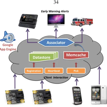
3.1 The CSN system collects performs decentralized anomaly detection by processing pick messages from low-cost sensors and smartphone accelerometers. Data is processed in a web application built on Google’s App Engine. Data products, such as alerts and shake maps, may be issued to the community or emergency responders. . . 34 3.2 CSN volunteers contribute data from low-cost accelerometers (above) and from Android
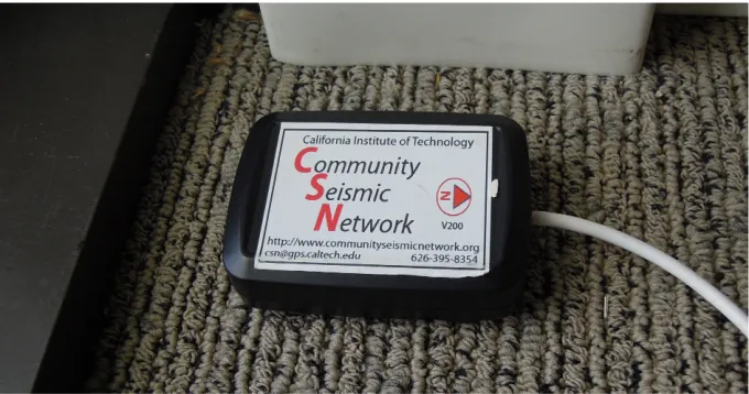
smart-phones via a CSN app. . . 35 3.3 Map of locations where measurements have been reported from during our pilot deployment of
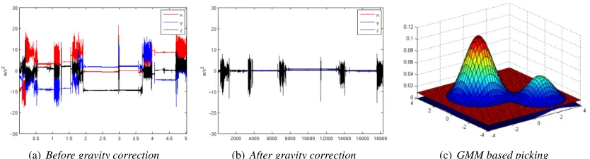
CSN. . . 35 3.4 A low-cost USB accelerometer manufactured by Phidget, Inc. . . 36 3.5 CSN-Droid app architecture . . . 37 3.6 (a) 5 hours of recording three-axis accelerometer data during normal cell phone use. (b) Data
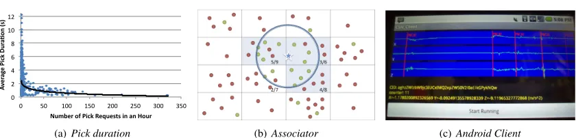
from (a) after removing gravity and appropriate signal rotation. (c) Illustration of the density estimation based picking algorithm. The red plane shows an operating threshold. Acceleration patterns for which the density does not exceed the threshold result in a pick. . . 38 3.7 (a) Average duration of a pick request as a function of system load. (b) Model of dispersed
sensors using a hash to a uniform grid to establish proximity. (c) A picture of the CSN android client in debug mode, capturing picks. . . 41 3.8 (a,b) Sensor level ROC curves for magnitude 5-5.5 events, for Android (a) and Phidget (b)
sensors. In (c-d), the system-level false positive rate is constrained to 1 per year, and the achievable detection performance is shown: (c) Detection rate as a function of the number of sensors in a 20 km×20 km cell. We show the achievable performance guaranteeing one false positive per year, while varying the number of cells covered. (d,e) Detection performance for one cell, depending on the number of phones and Phidgets. (f) Actual detection performance for the Baja event. Note that our approach outperforms classical hypothesis testing, and closely matches the predicted performance. . . 43 3.9 Experimental setup for playing back historic earthquakes on a shaketable, and testing their
Abstract
Smartphones and other powerful sensor-equipped consumer devices make it possible to sense the physical world at an unprecedented scale. Nearly 2 million Android and iOS devices are activated every day, each carrying numerous sensors and a high-speed internet connection. Whereas traditional sensor networks have typicallydeployeda fixed number of devices to sense a particular phenomena, community networks cangrow as additional participants choose to install apps and join the network. In principle, this allows networks of thousands or millions of sensors to be created quickly and at low cost. However, making reliable inferences about the world using so many community sensors involves several challenges, including scalability, data quality, mobility, and user privacy.
Chapter 1
Introduction
In the last several years, mobile computing has drastically reshaped the way that people produce and access information. While it is easy to think of mobile devices simply assmallercomputers, smart devices like phones and tablets also possess an array of sensors - such as gyroscopes, cameras, accelerometers, and compasses - not present on traditional computers. These sensors are commonly used as additional forms of user input, but can be used more broadly to sense many aspects of the user’s immediate environment. In fact, a variety of recent commercial apps and products make use of or supplement these mobile sensors, including Google Glass, the Jawbone activity tracking wristband, the Nest home thermostat, and the FitBit. While the immediate intent of these products is personal sensing, the same technology is equally applicable to sensing city-wide or global environments.
Recently, the field ofCommunity Sensinghas emerged to study how networks of community-owned or operated devices can be used to sense the physical environment. For example, several recent sensing projects seek to partner with the owners of smartphones and other consumer devices to collect, share, and act on sensor data about phenomena that impact the community. Coupled to cloud computing platforms, such projects can reach an immense scale previously beyond the reach of sensor networks [10]. Current applications of community and participatory sensing include:
• Understanding traffic flows and monitoring road conditions [33, 61, 39, 8, 44, 31]
• Identifying sources of pollution [4, 1, 64]
• Monitoring public health [45, 42, 51]
• Responding to natural disasters like hurricanes, floods, and earthquakes [14, 20, 22, 34]
Scale. The volume of raw data that can be produced by a community network is astounding by any standard. Smartphones and other consumer devices often have multiple sensors, and can produce continuous streams of GPS position, acceleration, rotation, audio, and video data. While events of interest (e.g. traffic accidents, earthquakes, disease outbreaks) may be rare, devices must monitor continuously in order to detect them. Beyond obvious data heavyweights like video, rapidly monitoring even a single accelerometer or microphone produces hundreds of megabytes per day. Community sensing makes possible networks containing tens of thousands or millions of devices. For example, equipping taxi cabs with GPS devices or air quality sensors could easily yield a network of 50,000 sensors in a city like Beijing [71]. At these scales, even collecting a small set of summary statistics becomes daunting: if 500,000 sensors reported a brief status update once per minute, the total number of messages would rival the daily load in the Twitter network.
Non-traditional sensors. Community devices are also a different breed of sensor than those used in traditional scientific and industrial applications. Beyond simply being lower in accuracy (and cost) than “professional” sensors, community sensors are coupled to the individuals who own them. As a result, community sensors are often mobile, intermittently available, and directly experience the unique environment of an individual’s home, workplace, or pocket.
Complex Phenomena. By enabling sensor networks that densely cover cities, community sensors make it possible to measure and act on a range of important phenomena, including traffic patterns, pollution, and natural disasters. However, due to the previous lack of fine-grained data about these phenomena, these systems must simultaneously learn about the phenomena they are built to act upon. For example, a community seismic network may need to use measurements of frequent smaller quakes in order to obtain the models of ground composition needed to accurately estimate damage during rare, large quakes.
1.1
Main Contributions
The second contribution is a detailed study of earthquake detection in a community network of Android smartphones and other consumer sensors. Published in IPSN asThe Next Big One: Detecting Earthquakes and Other Rare Events from Community-based Sensors[22], this work presents the CaltechCommunity Seismic Network(CSN), a distributed system comprised of an Android app, a desktop client, and a Google App Engine cloud application. In contrast to many environmental sensing networks, a seismic network may experience long periods of time without observing the object of interest (i.e. a dangerously large earthquake). Consequently, earthquake monitoring is a task ofdetecting rare events. We describe how CSN uses distributed anomaly detection to transmit observations of potential earthquakes, while limiting bandwidth usage during the usual quiescent periods. This concept is implemented by the CSN-Droid Android app, and is evaluated with shake table experiments and simulations of historic earthquakes.
1.2
Related work
The work in this thesis draws on several fields of research. In addition to the community sensing research outlined above, there is also a significant amount of research on sensor selection and submodular optimization. The Caltech Community Seismic Network should be viewed in the context of several recent community-oriented seismic sensing projects, and in the context of recent developments in earthquake early warning systems. The problem of detecting spatial events using community sensors is directly related to a large body of work in decentralized detection and anomaly detection.
Sensor selection. The problem of deciding when to selectively turn on sensors in sensor networks in order to conserve power was first discussed by [57] and [73]. Many approaches for optimizing sensor placements and selection assume that sensors have a fixed region [32, 29, 6]. These regions are usually convex or even circular. Further, it is assumed that everything within a region can be perfectly observed, and everything outside cannot be measured by the sensors. For complex applications such as environmental monitoring, these assumptions are unrealistic, and the direct optimization of prediction accuracy is desired. The problem of selecting observations for monitoring spatial phenomena has been investigated extensively in geostatistics [15], and more generally (Bayesian) experimental design [11]. Several approaches have been proposed to activate sensors in order to minimize uncertainty [73] or prediction error [19]. However, these approaches do not have performance guarantees. Submodularity has been used to analyze algorithms for placing [38] or selecting [68] a fixed set of sensors. These approaches however assume that the model is known in advance.
Seismic networks. In addition to CSN, several other projects are exploring non-traditional seismic networks. Perhaps the most closely related system is the QuakeCatcher network [14]. While QuakeCatcher shares the use of MEMS accelerometers in USB devices and laptops, our system differs in its use of algorithms designed to execute efficiently on cloud computing systems and statistical algorithms for detecting rare events, particularly with heterogeneous sensors including mobile phones (which create far more complex statistical challenges). Kapoor et al. [34] analyze the increase in call volume after or during an event to detect earthquakes. Another related effort is the NetQuakes project [63], which deploys more expensive stand-alone seismographs with the help of community participation. Our CSN Phidget sensors achieve different tradeoffs between cost and accuracy. Several Earthquake Early Warning (EEW) systems have been developed to process data from existing sparse networks of high-fidelity seismic sensors (such as the Southern California Seismic Network). The Virtual Seismologist [16] applies a Bayesian approach to EEW, using prior information and seismic models to estimate the magnitude and location of an earthquake as sources of information arrive. ElarmS [3] uses the frequency content of initial P-wave measurements from sensors closest to the epicenter, and applies an attenuation function to estimate ground acceleration at further locations. We view our approach of community seismic networking as fully complementary to these efforts by providing a higher density of sensors and greater chance of measurements near to the epicenter. Our experiments provide encouraging results on the performance improvements that can be obtained by adding community sensors to an existing deployment of sparse but high quality sensors.
Decentralized detection. There has been a great deal of work in decentralized detection. The classical hierarchical hypothesis testing approach has been analyzed by Tsitsiklis [62]. Chamberland et al. [12] study classical hierarchical hypothesis testing under bandwidth constraints. Their goal is to minimizes the probability of error, under constraint on total network bandwidth. Wittenburg et al. [69] study distributed event detection in WSN. In contrast to the work above, their approach is distributed rather than decentralized: nearby nodes collaborate by exchanging feature vectors with neighbors before making decision. Their approach requires a training phase, providing examples of events that should be detected. Martinic et al. [43] also study distributed detection on multi-hop networks. Nodes are clustered into cells, and the observations within a cell are compared against a user-supplied “event signature” (a general query on the cell’s values) at the cell’s leader node (cluster head).
The communication requirements of the last two approaches are difficult to meet in community sensing applications, since sensors may not be able to communicate with their neighbors due to privacy and security restrictions. Both approaches require prior models (training data providing examples of events that should be detected, or appropriately formed queries) that may not be available in the seismic monitoring domain.
the idea of using GMMs for anomaly detection could be extended to learn, for each phone, a GMM that adapts to non-stationary sources of data.
Davy et al. [18] develop an online approach for anomaly detection using online Support Vector machines. One of their experiments is to detect anomalies in accelerometer recordings of industrial equipment. They use produce frequency-based (spectrogram) features, similar to the features we use. However, their approach assumes the centralized setting.
Chapter 2
Online Learning for Distributed Sensor
Selection
Community networks of consumer devices make it possible to build sensor networks at very large scale, yet efficiently operating such a network will require selectively gathering only a small percentage of the total sensor data. As an illustration, a single smartphone can easily produce hundreds of megabytes of sensor data, even if video data is not included. Transmitting this data from each device is both a burden on the device bandwidth and power, but also a burden on the central server that must process or store this information.
Sensor selectionis one strategy for reducing the burden of data collection, whereby individual sensors are activated at specific points in time in order to obtain the most useful information from the network (e.g., accurate predictions at unobserved locations) while also minimizing power consumption. Sensor selection is a key challenge in deploying sensor networks for real-world applications such as environmental monitoring [38], building automation [56]. The problem has received considerable attention [2, 73, 19], and algorithms with performance guarantees have been developed [2, 35]. However, many of the existing approaches make simplifying assumptions. Many approaches assume (1) that the sensors can perfectly observe a particular sensing region, and nothing outside the region [2]. This assumption does not allow us to model settings where multiple noisy sensors can help each other obtain better predictions. There are also approaches that base their notion of utility on more detailed models, such as improvement in prediction accuracy w.r.t. some statistical model [19] or detection performance [37]. However, most of these approaches make two crucial assumptions: (2) The model, upon which the optimization is based, is known in advance (e.g., based on domain knowledge or data from a pilot deployment) and (3), a centralized optimization selects the sensors (i.e., some centralized processor selects the sensors which obtain highest utility w.r.t. the model). We are not aware of any approach that simultaneously addresses the three main challenges (1), (2) and (3) above and still provides theoretical guarantees.
few sensors have been activated so far, and less if many sensors have already been activated. Our algorithm applies to any setting where the true objective is submodular [48], thus capturing a variety of realistic sensor models. Secondly, our algorithm does not require the model to be specified in advance: it learns to optimize the objective function in an online manner. Lastly, the algorithm is distributed; the sensors decide whether to activate themselves based on local information. We analyze our algorithm in the no-regret model, proving convergence properties similar to the best bounds for any centralized solution.
A bandit approach toward sensor selection. At the heart of our approach is a novel distributed algorithm for multiarmed bandit (MAB) problems. In the classical multiarmed bandit [54] setting, we picture a slot machine with multiple arms, where each arm generates a random payoff with unknown mean. Our goal is to devise a strategy for pulling arms to maximize the total reward accrued. The difference between the optimal arm’s payoff and the obtained payoff is called theregret. Known algorithms can achieve average per-round regret ofO(√nlogn/√T)wherenis the number of arms, andTthe number of rounds (see e.g. the survey of [25]). Suppose we would like to, at every time step, selectksensors. The sensor selection problem can then be cast as a multiarmed bandit problem, where there is one arm for each possible set ofksensors, and the payoff is the accrued utility for the selected set. Since the number of possible sets, and thus the number of arms, is exponentially large, the resulting regret bound isO(nk/2√logn/√T), i.e., exponential ink. However, when the utility function is submodular, the payoffs of these arms are correlated. Recent results [59] show that this correlation due to submodularity can be exploited by reducing thenk-armed bandit problem tokseparate
n-armed bandit problems, with only a bounded loss in performance.
Existing bandit algorithms, such as the widely used EXP3 algorithm [5], are centralized in nature. Consequently, the key challenge in distributed online submodular sensing is how to devise a distributed bandit algorithm. In Sec. 2.3 and 2.4, we develop a distributed variant of EXP3 using novel algorithms to sample from and update a probability distribution in a distributed way. Roughly, we develop a scheme where each sensor maintains its own weight, and activates itselfindependently from all other sensorspurely depending on this weight.
Observation specific selection. A shortcoming of centralized sensor selection is that the individual sensors’ current measurements are not considered in the selection process. In many applications, obtaining sensor measurements is less costly than transmitting the measurements across the network. For example, cell phones used in participatory sensing [9] can inexpensively obtain measurements on a regular basis, but it is expensive to constantly communicate measurements over the network. In Sec. 2.5, we extend our distributed selection algorithm to activate sensors depending on their observations, and analyze the tradeoff between power consumption and the utility obtained under observation specific activation.
Communication models. We analyze our algorithms under two models of communication cost: In the
model, messages can only be between a sensor and the base station, and each message has unit cost. In Sec. 2.3 we formulate and analyze a distributed algorithm for sensor selection under the simpler broadcast model. Then, in Sec. 2.4 we show how the algorithm can be extended to the star network model.
Our main contributions.
• Distributed EXP3, a novel distributed implementation of the classic multiarmed bandit algorithm. • Distributed Online Greedy (DOG) and LAZYDOG, novel algorithms for distributed online sensor
selection, which apply to many settings, only requiring the utility function to be submodular. • OD-DOG, an extension of DOG to allow for observation-dependent selection.
• We analyze our algorithm in the no-regret model and prove that it attains the optimal regret bounds
attainable by any efficient centralized algorithm.
• We evaluate our approach on several real-world sensing tasks including monitoring a 12,527 node
network.
2.1
Sensor Selection
We now formalize the sensor selection problem. Suppose a network of sensors has been deployed at a set of locationsV with the task of monitoring some phenomenon (e.g., temperature in a building). Constraints on communication bandwidth or battery power typically require us to select a subsetAof these sensors for activation, according to some utility function. The activated sensors then send their data to a server (base station). We first review the traditional offline setting where the utility function is specified in advance, illustrating how submodularity allows us to obtain provably near-optimal selections. We then address the more challenging setting where the utility function must be learned from data in an online manner.
2.1.1
The Offline Sensor Selection Problem
A standard offline sensor selection algorithm chooses a set of sensors that maximizes a known sensing quality objective functionf(A), subject to some constraints, e.g., on the number of activated sensors. One possible choice for the sensing quality is based on prediction accuracy (we will discuss other possible choices later on). In many applications, measurements are correlated across space, which allows us to make predictions at the unobserved locations. For example, prior work [19] has considered the setting where a random variableXsis associated with every locations∈V, and a joint probability distributionP(XV)models the
correlation between sensor values. Here,XV = [X1, . . . ,Xn]is the random vector over all measurements.
If some measurementsXA = xAare obtained at a subset of locations, then the conditional distribution
P(XV\A| XA=xA)allows predictions at the unobserved locations, e.g., by predictingE[XV\A| XA=xA].
is the mean squared prediction error,
MSE(XV\A|xA) =
1
n X
s∈V\A
E[(Xs−E[Xs|xA])2|xA].
In general, the measurementsxAthat sensorsAwill make is not known in advance. Thus, we can base our
optimization on theexpected mean squared prediction error,
EMSE(A) =
Z
dp(xA) MSE(XV\A|xA).
Equivalently, we can maximize thereductionin mean squared prediction error,
fEMSE(A) = EMSE(∅)−EMSE(A).
By definition, fEMSE(∅) = 0, i.e., no sensors obtain no utility. Furthermore, fEMSE is monotonic: if A ⊆ B ⊆V, thenfEMSE(A)≤fEMSE(B), i.e., adding more sensors always helps. That means,fEMSEis
maximized by the set of all sensorsV. However, in practice, we would like to only select a small set of, e.g., at mostksensors due to bandwidth and power constraints:
A∗= arg max
A
fEMSE(A)s.t.|A| ≤k.
Unfortunately, this optimization problem is NP-hard, so we cannot expect to efficiently find the optimal solution. Fortunately, it can be shown [17] that in many settings1, the functionfEMSEsatisfies an intuitive
diminishing returns property called submodularity. A set functionf : 2V →Ris calledsubmodularif, for
allA ⊆ B ⊆V ands∈V \ Bit holds thatf(A ∪ {s})−f(A)≥f(B ∪ {s})−f(B). Many other natural objective functions for sensor selection satisfy submodularity as well [36]. For example, thesensing region model wherefREG(A)is the total area covered by all sensorsAis submodular. Thedetectionmodel where
fDET(A)counts the expected number of targets detected by sensorsAis submodular as well.
A fundamental result of Nemhauser et al. [48] is that for monotone submodular functions, a simple greedy algorithm, which starts with the empty setA0=∅and iteratively adds the element
sk = arg max s∈V\Ak−1
f(Ak−1∪ {s}); Ak=Ak−1∪ {sk}
which maximally improves the utility obtains a near-optimal solution: For the setAkit holds that
f(Ak)≥(1−1/e) max
|A|≤k
f(A),
One fundamental problem with this offline approach is that it requires the functionf to be specified in advance, i.e., before running the greedy algorithm. For the functionfEMSE, this means that the probabilistic
modelP(XV)needs to be known in advance. While for some applications some prior data, e.g., from pilot
deployments, may be accessible, very often no such prior data is available. This leads to a “chicken-and-egg” problem, where sensors need to be activated to collect data in order to learn a model, but also the model is required to inform the sensor selection. This is akin to the “exploration–exploitation tradeoff” in reinforcement learning [5], where an agent needs to decide whether to explore and gather information about effectiveness of an action, or to exploit, i.e., choose actions known to be effective. In the following, we devise an online monitoring scheme based on this analogy.
2.1.2
The Online Sensor Selection Problem
We now consider the more challenging problem where the objective function is not specified in advance, and needs to be learned during the monitoring task. We assume that we intend to monitor the environment for a numberT of time steps (rounds). In each roundt, a setStof sensors is selected, and these sensors transmit
their measurements to a server (base station). The server then determines a sensing qualityft(St)quantifying
the utility obtained from the resulting analysis. For example, if our goal is spatial prediction, the server would build a model based on the previously collected sensor data, pick a random sensors, make prediction for the variableXs, and then compare the predictionµswith the sensor readingxs. The errorft=σ2s−(µs−xs)2
is an unbiased estimate of the reduction in EMSE. In the following analysis, we will only assume that the objective functionsftare bounded (w.l.o.g., take values in[0,1]), monotone, and submodular, and that we
have some way of computingft(S)for any subset of sensorsS. Our goal is to maximize the total reward
obtained by the system overT rounds,PT
t=1ft(St).
We seek to develop a protocol for selecting the setsStof sensors at each round, such that after a small
number of rounds the average performance of our online algorithm converges to the same performance of the offline strategy (that knows the objective functions). We thus compare our protocol against all strategies that can select a fixed set ofksensors for use in all of the rounds; the best such strategy obtains reward
maxS⊆V:|S|≤kP T
t=1ft(S). The difference between this quantity and what our protocol obtains is known as
itsregret, and an algorithm is said to beno-regretif its average regret tends to zero (or less)2asT → ∞.
Whenk= 1, our problem is simply the well-studiedmultiarmed bandit(MAB) problem, for which many no-regret algorithms are known [25]. For generalk, because the average of several submodular functions remains submodular, we can apply the result of Nemhauseret al. [48] (cf., Sec. 2.1.1) to prove that a simple greedy algorithm obtains a(1−1/e)approximation to the optimal offline solution. This is closely related to the problem of maximizing a monotone submodular function subject to a cardinality constraint. Nemhauseret al. [48] showed that for the latter problem the simply greedy algorithm obtains a(1−1/e)approximation, and Feige [24] showed that this is optimal in the sense that obtaining a
2Formally, ifR
(1−1/e+)approximation for any >0is NP-hard. These facts suggest that we cannot expect any efficient online algorithm to converge to a solution better than
(1−1/e) maxS⊆V:|S|≤kP T
t=1ft(S). We therefore define the(1−1/e)-regret of a sequence of (possibly
random) sets{St}Tt=1as
RT := (1−1/e)· max S⊆V:|S|≤k
T
X
t=1
ft(S) − T
X
t=1
E[ft(St)]
where the expectation is taken over the distribution for eachSt. We say an online algorithm producing a
sequence of sets hasno-(1−1/e)-regretiflim supT→∞RTT ≤0.
2.2
Centralized Online Sensor Selection
Before developing the distributed algorithm for online sensor selection, we will first review a centralized algorithm which is guaranteed to achieve no(1−1/e)-regret. In Sec. 2.3 we will show how this centralized algorithm can be implemented efficiently in a distributed manner. This algorithm starts with the greedy algorithm for a known submodular function mentioned in Sec. 2.1.1, and adapts it to the online setting. Doing so requires an online algorithm for selecting asinglesensor as a subroutine, and we review such an algorithm before discussing the centralized algorithm for selecting multiple sensors in Sec. 2.2.1.
Let us first consider the case where k = 1, i.e., we would like to select one sensor at each round. This simpler problem can be interpreted as an instance of the multiarmed bandit problem (as introduced in Sec. 2.1.2), where we have one arm for each possible sensor. In this case, the EXP3 algorithm [5] is a centralized solution for no-regret single sensor selection. EXP3 works as follows: It is parameterized by a learning rateη, and anexploration probabilityγ. It maintains a set of weightsws, one for each arm (sensor)s,
initialized to 1. At every roundt, it will select each armswith probability
ps= (1−γ)
ws
P
s0ws0
+γ
n,
i.e., with probabilityγit explores, picking an arm uniformly at random, and with probability(1−γ)it exploits, picking an armswith probability proportional to its weightws. Once an armshas been selected, a feedback
r=ft({s})is obtained, and the weightwsis updated to
ws←wsexp(ηr/ps).
Auer et al. [5] showed that with appropriately chosen learning rateηand exploration probabilityγit holds that the cumulative regretRT of EXP3 isO(
√
2.2.1
Selecting Multiple Sensors?
In principle, we could interpret the sensor selection problem as a nk-armed bandit problem, and apply existing no-regret algorithms such as EXP3. Unfortunately, this approach does not scale, since the number of arms grows exponentially withk. However, in contrast to the traditional multiarmed bandit problem, where the arms are assumed to have independent payoffs, in the sensor selection case, the utility function is submodular and thus the payoffs are correlated across different sets. Recently, Streeter and Golovin showed how this submodularity can be exploited, and developed a no-(1−1/e)-regret algorithm for online maximization of submodular functions [59].
The key idea behind their algorithm, OGunit, is to turn the offline greedy algorithm into an online algorithm
by replacing the greedy selection of the elementskthat maximizes the benefitsk= arg maxsf({s1, ..., sk−1}∪
{s})by a bandit algorithm. As shown in the pseudocode below, OGUNITmaintainskbandit algorithms, one
for each sensor to be selected. At each roundt, it selectsksensors according to the choices of thekbandit algorithmsEi3. Once the elements have been selected, theithbandit algorithmEireceives as feedback the
incremental benefitft(s1, . . . , si)−ft(s1, . . . , si−1), i.e., how much additional utility is obtained by adding
sensorsito the set of already selected sensors. Below we define[m] :={1,2, . . . , m}.
Algorithm OGUNITfrom [59]:
Initializekmultiarmed bandit algorithmsE1,E2, . . . ,Ek,
each with action setV. For each roundt∈[T]
For each stagei∈[k]in parallel Eiselects an actionvti
For eachi∈[k]in parallel
feedbackft(vjt:j≤i )−ft(vjt:j < i )toEi.
OutputSt={at1, a
t
2, . . . , a
t k}.
In [58] it is shown that OGUNIThas a 1−1
e
-regret bound ofO(kR)in this feedback model assuming each Eihas expected regret at mostR. Thus, when using EXP3 as a subroutine, OGUNIThas no-(1−1/e)-regret.
Unfortunately, EXP3 (and in fact all MAB algorithms with no-regret guarantees for non-stochastic reward functions) require sampling from some distribution with weights associated with the sensors. Ifnis small, we could simply store these weights on the server, and run the bandit algorithmsEithere. However, this solution
does not scale to large numbers of sensors. Thus the key problem for online sensor selection is to develop a multiarmed bandit algorithm which implementsdistributed samplingacross the network, with minimal overhead of communication. In addition, the algorithm needs to be able to maintain the distributions (the weights) associated with eachEiin a distributed fashion.
2.3
Distributed Online Sensor Selection
We will now develop DOG, an efficient algorithm for distributed online sensor selection. For now we make the following assumptions:
1. Each sensorv∈V is able to compute its contribution to the utilityft(S∪ {v})−ft(S), whereSare a
subset of sensors that have already been selected.
2. Each sensor can broadcast to all other sensors.
3. The sensors have calibrated clocks and unique, linearly ordered identifiers.
These assumptions are reasonable in many applications: (1) In target detection, for example, the objective functionft(S)counts the number of targets detected by the sensorsS. Once previously selected sensors have
broadcasted which targets they detected, the new sensorscan determine how many additional targets have been detected. Similarly, in statistical estimation, one sensor (or a small number of sensors) randomly activates each round and broadcasts its value. After sensorsShave been selected and announced their measurements, the new sensorscan then compute the improvement in prediction accuracy over the previously collected data. (2) The assumption that broadcasts are possible may be realistic for dense deployments and fairly long range transmissions. In Sec. 2.4 we will show how assumptions (1) and (2) can be relaxed.
As we have seen in Sec. 2.2, the key insight in developing a centralized algorithm for online selection is to replace the greedy selection of the sensor which maximally improves the total utility over the set of previously selected sensors by a bandit algorithm. Thus, a natural approach for developing a distributed algorithm for sensor selection is to first consider the single sensor case.
2.3.1
Distributed Selection of a Single Sensor
A naive distributed sampling scheme. A naive distributed algorithm would be to let each sensor keep track of all activation probabilitiesp. Then, one sensor (e.g., with the lowest identifier) would broadcast a single random numberuuniformly distributed in[0,1], and the sensorvfor whichPv−1
i=1pi≤u < Pv
i=1piwould
activate. However, for large sensor network deployments, this algorithm would require each sensor to store a large amount of global information (all activation probabilitiesp). Instead, each sensorvcould store only their own probability masspv; the sensors would then, in order of their identifiers, broadcast their probabilitiespv,
and stop once the sum of the probabilities exceedsu. This approach only requires a constant amount of local information, but requires an impracticalΘ(n)messages to be sent, and sent sequentially overΘ(n)time steps.
Distributed multinomial sampling. In this section we present a protocol that requires onlyO(1)messages in expectation, and only a constant amount of local information.
For a sampling procedure with input distributionp, we letpˆdenote the resulting distribution, where in all cases at most one sensor is selected, and nothing is selected with probability1−P
vpˆv. A simple approach
towards distributed sampling would be to activate each sensorv ∈V independentlyfrom each other with probabilitypv. While in expectation, exactly one sensor is activated, with probabilityQv(1−pv)>0no
sensor is activated; also since sensors are activated independently, there is a nonzero probability that more than one sensor is activated. Using a synchronized clock, the sensors could determine if no sensor is activated. In this case, they could simply repeat the selection procedure until at least one sensor is activated. One naive approach would be to repeat the selection procedure until exactly one sensor is activated. However with two sensors andp1 =ε, p2 = 1−εthis algorithm yieldspˆ1=ε2/(1−2ε+ 2ε2) =O(ε2), so the first sensor
is severely underrepresented. Another simple protocol would be to select exactly one sensor uniformly at random from the set of activated sensors, which can be implemented using few messages.
The Simple Protocol:
For each sensorvin parallel SampleXv ∼Bernoulli(pv).
If(Xv = 1),Xvactivates.
All active sensorsScoordinate to select a single sen-sor uniformly at random fromS, e.g., by electing the minimum ID sensor inSto do the sampling.
It is not hard to show that with this protocol, for all sensorsv,
ˆ
pv=pv·E 1
|S|
v∈S
≥pv/E[|S| |v∈S]≥pv/2
by appealing to Jensen’s inequality. Sincepˆv ≤ pv, we find that this simple protocol maintains a ratio
rv:= ˆpv/pv∈[12,1]. Unfortunately, this analysis is tight, as can be seen from the example with two sensors
To improve upon the simple protocol, first consider running it on an example withp1=p2=· · ·=pn=
1/n. Since the protocol behaves exactly the same under permutations of sensor labels, by symmetry we have
ˆ
p1= ˆp2 =· · ·= ˆpn, and thusri =rjfor alli, j. Now consider an input distributionpwhere there exists
integersNandk1, k2, . . . , knsuch thatpv=kv/Nfor allv. Replace eachvwithkvfictitious sensors, each
with probability mass1/N, and each with a label indicatingv. Run the simple protocol with the fictitious sensors, selecting a fictitious sensorv0, and then actually select the sensor indicated by the label ofv0. By symmetry this process selects each fictitious sensor with probability(1−β)/N, whereβis the probability that nothing at all is selected, and thus the process selects sensorvwith probabilitykv(1−β)/N= (1−β)pv
(since at most one fictitious sensor is ever selected).
We may thus consider the following improved protocol which incorporates the above idea, simulating this modification to the protocol exactly whenpv =kv/Nfor allv.
The Improved Protocol(N):
For each sensorvin parallel
SampleXv ∼Binomial(dN·pve,1/N).
If(Xv ≥1), then activate sensorv.
From the active sensorsS, select sensorvwith proba-bilityXv/Pv0∈SXv0.
This protocol ensures the ratiosrv:= ˆpv/pvare the same for all sensors, provided eachpvis a multiple
of1/N. Assuming the probabilities are rational, there will be a sufficiently largeN to satisfy this condition. To reduceβ := Pr[S=∅]in the simple protocol, we may sample each Xv fromBernoulli(α·pv)for
anyα ∈ [1, n]. The symmetry argument remains unchanged. This in turn suggests sampling Xv from
Binomial(dN·pve, α/N)in the improved protocol. Taking the limit asN → ∞, the binomial distribution
becomes Poisson, and we obtain the desired protocol.
The Poisson Multinomial Sampling (PMS) Protocol(α):
Same as the improved protocol, except each sensorvsamplesXv∼Poisson(αpv)
Straight-forward calculation shows that
Pr[S=∅] =Y
v
exp{−α·pv}= exp−
X
v
α·pv =e−α
LetCbe the number of messages. Then
E[C] = X
v
Pr[Xv≥1] =
X
v
(1−e−αpv)≤X
v
αpv=α
Here we have used linearity of expectation, and1 +x≤exfor allx∈
R. In summary, we have the following
Proposition 1. Fix any fixedpandα >0. The PMS Protocol always selects at most one sensor, ensures
∀v: Pr[vselected] = (1−e−α)pv
and requires no more thanαmessages in expectation.
In order to ensure that exactly one sensor is selected, wheneverS=∅we can simply rerun the protocol with fresh random seeds as many times as needed untilS is non-empty. Usingα= 1, this modification will require onlyO(1)messages in expectation and at mostO(logn)messages with high probability in the broadcast model. We can combine this protocol with EXP3 to get the following result.
Theorem 2. In the broadcast model, runningEXP3using the PMS Protocol withα= 1, and rerunning the
protocol whenever nothing is selected, yields exactly the same regret bound as standardEXP3, and in each round at moste/(e−1) + 2≈3.582messages are broadcast in expectation.
The regret bound for EXP3 isO(pOPTnlogn), whereOPTis the total reward of the best action. Our variant simulates EXP3, and thus has identical regret.
Remark. Running our variant of EXP3 requires that each sensor know the number of sensors,n, in order to compute its activation probability. If each sensorvhas only a reasonable estimate ofnvofn, however,
our algorithm still performs well. For example, it is possible to prove that if all of the sensors have the same estimatenv =cnfor some constantc >0, then the upper bound on expected regret,R(c), grows as
R(c)≈R(1)·max{c,1/c}. The expected number of activations in this case increases by at most 1
c −1
γ. In general underestimatingnleads to more activations, and underestimating or overestimatingncan lead to more regret. This graceful degradation of performance with respect to the error in estimatingnholds for all of our algorithms.
2.3.2
Distributed Online Greedy
We now use our single sensor selection algorithm to develop our main algorithm, the Distributed Online Greedy algorithm (DOG). It is based on the distributed implementation of EXP3 using the PMS Protocol. Suppose we would like to selectksensors at each roundt. Each sensorvmaintainskweightswv,1, . . . , wv,k
and normalizing constantsZv,1, . . . , Zv,k. The algorithm proceeds in k stages, synchronized using the
common clock. In stagei, a single sensor is selected using the PMS Protocol applied to the distribution
(1−γ)wv,i/Zv,i+γ/n. Suppose sensorsS ={v1, . . . , vi−1}have been selected in stages1throughi−1. The
sensorvselected at stageithen computes its local rewardsπv,iusing the utility functionft(S∪ {vi})−ft(S).
It then computes its new weight
and broadcasts the difference between its new and old weights∆v,i=w0v,i−wv,i. All sensors then update
theirithnormalizers usingZ
v,i←Zv,i+ ∆v,i. Fig. 1 presents the pseudo-code of the DOG algorithm. Thus
given Theorem12of [58] we have the following result about the DOG algorithm:
Theorem 3. TheDOGalgorithm selects, at each roundta setSt⊆V ofksensors such that
1
TE " T
X
t=1 ft(St)
#
≥ 1−
1
e
T |maxS|≤k T
X
t=1
ft(S)−O k
r nlogn
T !
.
In expectation, onlyO(k)messages are exchanged each round.
Algorithm 1:The Distributed Online Greedy Algorithm
Input: k∈N, a setV, andα, γ, η∈R>0. Reasonable defaults are anyα∈[1,ln|V|], andγ=η=
min1,(|V|ln|V|/g)1/2, wheregis a guess for the maximum cumulative reward of any single sensor [5].
Initializewv,i←1andZv,i← |V|for allv∈V,i∈[k]. Letρ(x, y) := (1−γ)xy+|Vγ|.
for eachroundt= 1,2,3, . . .do
InitializeSv,t ← ∅for eachvin parallel.
for eachstagei∈[k]do
for eachsensorv∈V in paralleldo repeat
SampleXv ∼Poisson(α·ρ(wv,i, Zv,i)).
if(Xv≥1)then
BroadcasthsampledXv,id(v)i; Receive messages from sensorsS. (Includev∈S
for convenience).
ifid(v) = minv0∈Sid(v0)then
Select exactly one elementvitfromSsuch that eachv0is selected with
probabilityXv0/P
u∈SXu.
Broadcasthselect id(vit)i.
Receive messagehselect id(vit)i.
ifid(v) = id(vit)then
Observeft(Sv,t+v);π←ft(Sv,t+v)−ft(Sv,t);
∆v←wv,i(exp{η·π/ρ(wv,i, Zv,i)} −1);Zv,i←Zv,i+ ∆v;
wv←wv+ ∆v; Broadcasthweight update∆v,id(v)i.
ifreceive messagehweight update∆,id(vit)ithen Sv,t←Sv,t∪ {vit};
Zv,i←Zv,i+ ∆;
;
untilvreceives a message of type hselect idi;
Output: At the end of each roundteach sensor has an identical local copySv,tof the selected setSt.
2.4
Communication to the cloud: The Star Network Model
In some applications, the assumption that sensors can broadcast messages to all sensors may be unrealistic. Furthermore, in some applications sensors may not be able to compute the marginal benefitsft(S∪{s})−ft(S)
our DOG algorithm, which replace the above assumptions by the assumption that there is a dedicated base station4available which computes utilities and which can send non-broadcast messages to individual sensors.
We make the following assumptions:
1. Every sensor stores its probability masspvwith it, and can only send messages to and receive messages
from the base station.
2. The base station is able, after receiving messages from a setSof sensors, to compute the utilityft(S)
and send this utility back to the active sensors.
These conditions arise, for example, when cell phones in participatory sensor networks can contact the base station, but due to privacy constraints cannot directly call other phones. We do not assume that the base station has access to all weights of the sensors – we will only require the base station to haveO(k+ logn)memory. In the fully distributed algorithm DOG that relies on broadcasts, it is easy for the sensors to maintain their normalizersZv,i, since they receive information about rewards from all selected sensors. The key challenge
when removing the broadcast assumption is to maintain the normalizers in an appropriate manner.
2.4.1
Lazy Renormalization & Distributed EXP3
EXP3 (and all MAB with no-regret guarantees against arbitrary reward functions) must maintain a distribution over actions, and update this distribution in response to feedback about the environment. In EXP3, each sensor
vrequires onlywv(t)and a normalizerZ(t) :=Pv0wv0(t)to computepv(t)5. The former changes only when vis selected. In the broadcast model the latter can simply be broadcast at the end of each round. In the star network model (or, more generally in multi-hop models), standard flooding echo aggregation techniques could be used to compute and distribute the new normalizer, though with high communication cost. We show that a lazy renormalization scheme can significantly reduce the amount of communication needed by a distributed bandit algorithmwithout altering its regret bounds whatsoever. Thus our lazy scheme is complementary to standard aggregation techniques.
Our lazy renormalization scheme for EXP3 works as follows. Each sensorvmaintains its weightwv(t)
and an estimateZv(t)forZ(t) :=Pv0wv0(t), Initially, wv(0) = 1andZv(0) = nfor allv. The central
server storesZ(t). Let
ρ(x, y) := (1−γ)x
y + γ n.
Each sensor then proceeds to activate as in the sampling procedure of Sec. 2.3.1 as if its probability mass in roundtwereqv=ρ(wv(t), Zv(t))instead of its true value ofρ(wv(t), Z(t)). A single sensor is selected by
the server with respect to the true valueZ(t), resulting in a selection from the desired distribution. Moreover,
4Though the existence of such a base station means the protocol is not completely distributed, it is realistic in sensor network
applications where the sensor data needs to be accumulated somewhere for analysis.
5We letx(t)denote the value of variablexat the start of roundt, to ease analysis. We do not actually need to store the historical
v’s estimateZv(t)is only updated on rounds when it communicates with the server under these circumstances.
This allows the estimated probabilities of all of the sensors to sum to more than one, but has the benefit of significantly reducing the communication cost in the star network model under certain assumptions. We call the resultDistributed EXP3, give its pseudocode for roundtin Fig. 2.
Since the sensors underestimate their normalizers, they may activate more frequently than in the broadcast model. Fortunately, the amount of “overactivation” remains bounded.
Theorem 4. The number of sensor activations in any round of the DistributedEXP3algorithm is at most
α+ (e−1)in expectation andO(α+ logn)with high probability, and the number of messages is at most twice the number of activations.
Unfortunately, there is still ane−αprobability of nothing being selected. To address this, we can set
α=clnnfor somec≥1, and if nothing is selected, transmit a message to each of thensensors to rerun the protocol.
Corollary 5. There is a distributed implementation of EXP3that always selects a sensor in each round, has the same regret bounds as standardEXP3, ensures that the number of sensor activations in any round is at mostlnn+O(1)in expectation orO(logn)with high probability, and in which the number of messages is at most twice the number of activations.
2.4.2
Lazy Renormalization
Once we have the distributed EXP3 variant described above, we can use it for the bandit subroutines in the OGUNITalgorithm (cf.Sec. 2.2.1). We call the result theLAZYDOG algorithm, due to its use of lazy renormalization. The lazy distributed EXP3 still samples sensors from the same distribution as the regular distributed EXP3, soLAZYDOG has precisely the same performance guarantees with respect toP
tft(St)as
DOG. It works in the star network communication model, and requires few messages or sensor activations. Corollary 5 immediately implies the following result.
Corollary 6. The number of sensors that activate each round inLAZYDOGis at mostklnn+O(k)in
expectation andO(klogn)with high probability, the number of messages is at most twice the number of activations, and the(1−1/e)-regret of LAZYDOGis the same asDOG.
2.5
Observation-dependent sampling
Theorem 3 states that DOG is guaranteed to do nearly as well as the offline greedy algorithm run on an instance with objective functionfΣ:=Ptft. Thus the reward of DOG is asymptotically near-optimal on
Algorithm 2:Distributed EXP3: the PMS Protocol(α) with lazy renormalization, applied to EXP3
Input: Parametersα, η, γ∈R>0, sensor setV.
Letρ(x, y) := (1−γ)xy +|Vγ|. Sensors:
foreachsensorvin paralleldo
Samplervuniformly at random from[0,1].
if(rv≥1−α·ρ(wv(t), Zv(t))then
Sendhrv, wv(t)ito the server.
Receive messagehZ, wifrom server.
Zv(t+ 1)←Z;wv(t+ 1)←w.
else Zv(t+ 1)←Zv(t);wv(t+ 1)←wv(t).
; Server:
Receive messages from a setSof sensors.
ifS=∅thenSelect nothing and wait for next round.;
else foreachsensorv∈Sdo
Yv←min{x:Pr[X≤x]≥rv}, whereX ∼Poisson(α·ρ(wv(t), Z(t))).
Selectvwith probabilityYv/Pv0∈SYv0.
Observe the payoffπfor the selected sensorv∗;wv∗(t+ 1)←wv∗(t)·exp{ηπ/ρ(wv∗(t), Z(t))}; Z(t+ 1)←Z(t) +wv∗(t+ 1)−wv∗(t);
for eachv∈S\v∗do wv(t+ 1)←wv(t);
;
for eachv∈Sdo SendhZ(t+1), wv(t+1)itov.
; ;
with significant events, even if the nearest sensors typically report “boring” readings that contribute very little to the objective function. For now, suppose that we are only running a single MAB instance to select a single sensor in each round. If we have access to a black-box for evaluatingfton roundt, then we can perform well
on atypical rounds at the cost of some additional communication by having each sensorvtake a local reading of its environment and estimate its payoff¯π=ft({v})if selected. This value, which serves as a measure
of how interesting its input is, can then be used to decide whether to boostv’s probability for reporting its sensor reading to the server. In the simplest case, we can imagine that eachvhas a thresholdτvsuch thatv
activates with probability1ifπ¯≥τv, and with its normal probability otherwise. In the case where we select
k >1sensors in each round, each sensor can have a threshold for each of thekstages, where in each stage it computes¯π=ft(S∪ {v})−ft(S)whereSis the set of currently selected sensors. Since the activation
probability only goes up, we can retain the performance guarantees of DOG if we are careful to adjust the feedback properly.
Ideally, we wish that the sensors learn what their thresholdsτv should be. We treat the selection ofτv
in each round as an online decision problem that eachvmust play. We construct a particular game that the sensors play, where the strategies are the thresholds (suitably discretized), there is anactivation costcvthatv
pays ifπ¯v ≥τv, and the payoffs are defined as follows: Letπv=ft(S∪ {v})−ft(S)be the marginal benefit
the current iteration of the game, and letmax π(A\v)
:= max (πv0 :v0∈A\ {v}). The particular reward
functionψvwe choose for each sensorvfor each iteration of the game is
ψv(τ) =
cv−max πv−max π(A\v)
,0
if¯π < τ
max πv−max π(A\v)
,0
−cv if¯π≥τ
based on empirical performance. Thus, if a sensor activates (π¯≥τ), its payoff is the improvement over the best payoffπv0 among all sensorsv0 ∈ Aminus its activation cost. In case multiple sensors activate, the
highest reward is retained.
In the broadcast model where each sensor can compute its marginal benefit, we can use any standard no-regret algorithm for combining expert advice, such asRandomized Weighted Majority(WMR) [41], to play this game and obtain no regret guarantees6for selectingτ
v. In our context a sensor using WMR simply
maintains weightsw(τi) = exp (η·ψtotal(τi))for each possible thresholdτi, whereη > 0 is a learning
parameter, andψtotal(τi)is the total cumulative reward for playingτiin every round so far. On each step each
threshold is picked with probability proportional to its weight. In the more restricted star network model, we can use a modification of WMR that feeds back unbiased estimates forψt(τi), the payoff to the sensor for
using a threshold ofτiin roundt, and thus obtains reasonably good estimates ofψtotal(τi)after many rounds.
We give pseudocode in Fig. 3. In it, we assume that an activated sensor can compute the reward of playing any threshold.
Algorithm 3:Selecting activation thresholds for a sensor
Input: parameterη >0, threshold set{τi:i∈[m]}
Initializew(τi)←1for alli∈[m].
for each roundt= 1,2, . . .do
Selectτiwith probabilityw(τi)/P m
j=1w(τj).
if sensor activatesthen
Letψ(τi)be the reward for playingτiin this round of the game. Letq(τi)be the total
probability of activation conditioned onτibeing selected (including the activation probability
that does not depend on local observations.)
for each thresholdτido
w(τi)←w(τi) exp (ηψ(τi)/q(τi)).
We incorporate these ideas into the DOG algorithm, to obtain what we call theObservation-Dependent Distributed Online Greedyalgorithm (OD-DOG). In the extreme case thatcv= 0for allvthe sensors will
soon set their thresholds so low that each sensor activates in each round. In this case OD-DOG will exactly simulate the offline greedy algorithm run on each round. In other words, if we letG(f)be the result of running the offline greedy algorithm on the problem
arg max{f(S) :S⊂V, |S| ≤k}
6We leave it as an open problem to determine if the outcome is close to optimal when all sensors play low regret strategies (i.e., is the
then OD-DOG will obtain a value ofP
tft(G(ft)); in contrast, DOG gets roughlyPtft(G(Ptft)), which
may be significantly smaller. Note that Feige’s result [24] implies that the former value is the best we can hope for from efficient algorithms (assuming P6=NP). Of course, querying each sensor in each round is impractical when querying sensors is expensive. In the other extreme case where cv = ∞for allv, OD-DOG will
simulate DOG after a brief learning phase. In general, by adjusting the activation costscvwe can smoothly
trade off the cost of sensor communication with the value of the resulting data.
2.6
Experiments in sensor selection
In this section, we evaluate our DOG algorithm on several real-world sensing problems.
2.6.1
Data Sets
Temperature data. In our first data set, we analyze temperature measurements from the network of 46 sensors deployed at Intel Research Berkeley. Our training data consisted of samples collected at 30 second intervals on 3 consecutive days (starting Feb. 28th 2004), the testing data consisted of the corresponding samples on the two following days. The objective functions used for this application are based on the expected reduction in mean squared prediction errorfEMSE, as introduced in Sec. 2.1.
Precipitation data. Our second data set consists of precipitation data collected during the years 1949 - 1994 in the states of Washington and Oregon [67]. Overall 167 regions of equal area, approximately 50 km apart, reported the daily precipitation. To ensure the data could be reasonably modeled using a Gaussian process we applied preprocessing as described in [38]. As objective functions we again use the expected reduction in mean squared prediction errorfEMSE.
picks the contamination strategy knowing our network deployment and selection algorithm). The algorithms developed here apply to such adversarial settings. We reproduce the experimental setup detailed in [37]. For each contamination eventi, we define a separate submodular objective functionfi(S)that measures the
expected population protected when detecting the contamination from sensorsS. In [37], Krause et al. showed that the functionsfi(A)are monotone submodular functions.
2.6.2
Convergence Experiments
In our first set of experiments, we analyzed the convergence of our DOG algorithm. For both the temperature [T] and precipitation [R] data sets, we first run the offline greedy algorithm using thefEMSEobjective function to pickk= 5sensors. We compare its performance to the DOG algorithm, where we feed back the same objective function at every round. We use an exploration probabilityγ= 0.01and a learning rate inversely proportional to the maximum achievable rewardfEMSE(V). Fig. 2.1(a) presents the results for the temperature data set. Note that even after only a small number of rounds (≈ 100), the algorithm obtains 95% of the
performance of the offline algorithm. After about 13,000 iterations, the algorithm obtains 99% of the offline performance, which is the best that can be expected with a.01exploration probability. Fig. 2.1(b) show the same experiment on the precipitation data set. In this more complex problem, after 100 iterations, 76% of the offline performance is obtained, which increases to 87% after 500,000 iterations.
2.6.3
Observation Dependent Activation
We also experimentally evaluate our OD-DOG algorithm with observation specific sensor activations. We choose different values for the activation costcv, which we vary as multiples of the total achievable reward.
The activation costcvlets us smoothly trade off the average number of sensors activating each round and the
0 1 2 3 4 5 x 10⁵ 9.4 9.5 9.6 9.7 9.8 9.9 iterations average reward Offline DOG
(a)[T] Convergence
0 1 2 3 4 5
x 105 0.35
0.4 0.45 0.5
iterations
average reward DOG Offline
(b)[R] Convergence
0 50 100 150 200 250 1.2 1.5 1.8 2.1 2.4 2.6 iterations
average reward (x10
7) C v=1 C v=0.1 C v=0.02 C v=0.005 C
v=0.0001 Offline
(c)[W] Constant Objective
0 100 200 300 400 500
0 2 4 6 8 10 12 14 iterations
average reward (x10
4)
C
v=0.07 Cv=0.26
Offline
Cv=0.005
Cv=0.0001
C v=1
[image:31.612.111.537.259.511.2](d)[W] Varying Objective
Chapter 3
Decentralized Anomaly Detection in
Community Networks
In contrast to the previous chapter which focused on repeatedly selecting sets of sensors to observe the same (or similar) environment, this chapter considers the problem of detecting sudden andrare events such as earthquakes or other disasters using data from a large community network. Due to the unavailability of data characterizing the rare events, the approach described here is based on anomaly detection. First, each sensor learns a model of normal sensor data (e.g., acceleration patterns experienced by smartphones under typical manipulation). Each sensor then independently detects unusual observations (which are considered unlikely with respect to the model), and notifies a central server, orfusion center. The fusion center then decides whether a rare event has occurred or not based on the received messages. Our approach is grounded in the theory of decentralized detection, and we characterize its performance accordingly. In particular, we show how sensors can learn decision rules that allow us to control system-level false positive rates and bound the amount of required communication in a principled manner while simultaneously maximizing the detection performance.
To better study the challenges and opportunities of community sensing, we implement our approach in theCommunity Seismic Network (CSN). The goal of the CSN system is to detect seismic motion using accelerometers in smartphones and other consumer devices (Figure 3.4), and issue real-time early-warning of seismic hazards. The duration of the warning is the time between a person or device receiving the alert and the onset of significant shaking; this duration depends on the distance between the location of initial shaking and the location of the receiving device, and on delays within the network and fusion center. Warnings of up to tens of seconds are possible [3], and even warnings of a few seconds help in stopping elevators, slowing trains, and closing gas valves. Since false alarms can have high costs, it is important to limit the false positive rate of the system.
change over time; for example, construction may start in some places and stop in others. With thousands of sensors, one cannot expect to know the precise characteristics of each sensor at each point in time; these characteristics have to be deduced by algorithms. A system that scales to tens of thousands or millions of sensors must limit the rate of message traffic so that it can be handled efficiently by the network and fusion center. For example, one million phones would produce approximately 30 Terabytes of accelerometer data each day. Another key challenge is to develop a system infrastructure that has low response time even under peak load (messages sent by millions of phones during an earthquake). Moreover, the Internet and computers in a quake zone are likely to fail with the onset of intensive shaking. So, data from sensors must be sent out to a distributed, resilient system that has data centers outside the quake zone. The CSN uses cloud-computing based sensor fusion to cope with these challenges. We report our initial experience with the CSN, and experimentally evaluate our detection approach based on data from a pilot deployment. Our results, including data from shaketable experiments that allow us to mechanically play back past earthquakes, indicate the effectiveness of our approach in distinguishing seismic motion from accelerations due to normal daily manipulation. They also provide evidence for the feasibility of earthquake early warning using a dense network of cell phones.
In summary, this chapter describes:
• a novel approach for online decentralized anomaly detection,
• a theoretical analysis, characterizing the performance of our detection approach,
• an implementation of our approach in the Community Seismic Network, involving smartphones, USB
MEMS accelerometers and cloud-computing based sensor fusion, and
• a detailed empirical evaluation of our approach characterizing the achievable detection performance
when using smartphones to detect earthquakes.
3.1
Problem Statement
We consider the problem of decentralized detection of rare events, such as earthquakes, under constraints on the number of messages sent by each sensor. Specifically, a set ofN sensors make repeated observations Xt= (X1,t, . . . , XN,t)from which we would like to detect the occurrence of an eventEt∈ {0,1}. Here,
Xs,tis the measurement of sensorsat timet, andEt= 1iff there is an event (e.g., an earthquake) at time
t. Xs,tmay be a scalar (e.g., acceleration), or a vector of features containing information about Fourier
frequencies, moments, etc. during a sliding window of data (see Section 3.4.2 for a discussion of features that we use in our system).
We are interested in the decentralized setting, where each sensorsanalyzes its measurementsXs,t, and
sends a messageMs,tto the fusion center. Here we will focus on binary messages (i.e., each sensor gets to
vote on whether there is an event or not). In this case,Ms,t= 1means that sensorsat timetestimates that an
event happened;Ms,t= 0means that sensorsat timetestimates that no event happened at that time. For
we only need to send messages (that we henceforth callpicks) forMs,t = 1; sending no message implies
Ms,t = 0. Based on the received messages, the fusion center then decides how to respond: It produces an
estimateEbt∈ {0,1}. IfEbt=Et, it makes the correct decision (true positiveifEt= 1ortrue negativeif
Et= 0). IfEbt= 0whenEt= 1, it missed an event and thus produced afalse negative. Similarly, ifEbt= 1
whenEt= 0, it produced afalse positive. False positives and false negatives can have very different costs. In
our earthquake example, a false positive could lead to incorrect warning messages sent out to the community and consequently lead to inappropriate execution of remedial measures. On the other hand, false negatives could lead to missed opportunities for protecting infrastructure and saving lives. In general, our goal will be to minimize the frequency of false negatives while constraining the (expected) frequency of false positives to a tolerable level (e.g., at most one false alarm per year).
Classical Decentralized Detection. How should each sensor, based on its measurementsXs,t, decide when
topick(sendMs,t= 1)? The traditional approach to decentralized detection assumes that we know how likely
particular observationsXs,tare, in case of an event occurring or not occurring. Thus, it assumes we have
access to the conditional probabilitiesP[Xs,t|Et= 0]andP[Xs,t|Et= 1]. In this case, under the common
assumptions that the sensors’ measurements are independent conditional on whether there is an event or not, it can be shown that the optimal strategy is to performhierarchical hypothesis testing[62]: we define two thresholdsτ, τ0, and letM
s,t= 1iff
P[Xs,t|Et= 1]
P[Xs,t|Et= 0]
≥τ. (3.1)
i.e., if the likelihood ratio exceedsτ. Similarly, the fusion center setsEbt= 1iff
Bin(St;p1;N)
Bin(St;p0;N)
≥τ0, (3.2)
whereSt=PsMs,tis the number of picks at timet;p`=P[Ms,t= 1|Et=`]is the sensor-level true (`=
1) and false (`= 0) positive rate respectively; andBin(·, p, N)is the probability mass function of the Binomial distribution. Asymptotically optimal decision performance in either a Bayesian or Neyman-Pearson framework can be obtained by using the decision rules (3.1) and (3.2) with proper choice of the thresholdsτandτ0[62].
There has also been work inquickest detectionorchange detection(cf., [52] for an overview), where the assumption is that there is some time pointt0at which the event occurs;Xs,twill be distributed according
toP[Xs,t|Et= 0]for allt < t0, and according toP[Xs,t|Et= 1]for allt≥t0. In change detection, the
system trades off waiting (gathering more data) and improved detection performance. However, in case of raretransientevents (such as earthquakes) that may occur repeatedly, the distributionsP[Xs,t|Et= 1]are
expected to change withtfort≥t0.
(i) Sensors are highly heterogeneous (i.e., the distributionsP[Xs,t|Et]are different for each sensors)
(ii) Since events are rare, we do not have sufficient data to obtain good models forP[Xs,t|Et= 1]
(iii) Bandwidth limitations may limit the amount of communication (e.g., number of picks sent).
Challenge (i) alone would not be problematic – classical decentralized detection can be extended to heterogeneous sensors, as long as we knowP[Xs,t|Et]. For the case where we do not knowP[Xs,t|Et],
but we have training examples (i.e., large collections of sensor data, annotated by whether an event is present or not), we can use techniques from nonparametric decentralized detection [49]. In the case of rare events, however, we may be able to collect large amounts of data forP[Xs,t|Et= 0](i.e., characterizing the sensors
in the no-event case), while still collecting extremely little (if any) data for estimatingP[Xs,t|Et= 1]. In our
case, we would need to collect data from cell phones experiencing seismic motion of earthquakes ranging in magnitude from three to ten on the Gutenberg-Richter scale, while resting on a table, being carried in a pocket, backpack, etc. Furthermore, even though we can collect much data forP[Xs,t|Et= 0], due to challenge (iii)
we may not be able to transmit all the data to the fusion center, but have to estimate this distribution locally, possibly with limited memory. We also want to choose decision rules that minimize the number of messages sent.
3.2
Online Decentralized Anomaly Detection
We now describe our approach to online, decentralized detection of anomalous events.
Assumptions. In the following, we adopt the assumption of classical decentralized detection that sensor observations are conditionally independent givenEt, and independent across time (i.e., the distributions
P[Xs,t|Et= 0]do not depend ont). For earthquake detection this assumption is reasonable (since most of
the noise is explained through independent measurement noise and user activity). While spatial correlation may be present, e.g., due to mass events such as rock concerts, it is expected to be relatively rare. Furthermore, if context about such events is available in advance, it can be taken into account. We defer treatment of spatial correlation to future work. We donotassume that the sensors are homogeneous (i.e.,P[Xs,t|Et= 0]may
depend ons). Our approach can be extended in a straightforward manner if the dependence ontis periodic (e.g., the background noise changes based on the time of day, or day within week).
Overview. The key idea behind our approach is that since sensors obtain a massive amount of normal data, they can accurately estimateP[Xs,t|Et= 0]purely based on their local observations. In our earthquake
monitoring example, the cell phones can collect data of acceleration experienced under normal operation (lying on a table, being carried in a backpack, etc.). Further, if we have hope of detecting earthquakes, the signal
Xs,tmust be sufficiently different from normal data (thusP[Xs,t|Et= 0]must be low whenEt= 1). This
![Figure 2.1: Experimental results on [T] Temperature data, [R] precipitation data and [W] water distribution network data.](https://thumb-us.123doks.com/thumbv2/123dok_us/8591820.863720/31.612.111.537.259.511/figure-experimental-results-temperature-precipitation-water-distribution-network.webp)