Optimization Techniques for Engineering Design

Optimization Techniques for Engineering Design

Dr. Kailas Chaudhary1

1

Professor Department of Mechanical Engineering Raj Engineering College Jodhpur, India

Abstract: This paper discusses the popular evolutionary optimization technique, Genetic Algorithm (GA)and Teaching-learning-based Optimization (TLBO) algorithm. It also covers the definitions of various parameters used by these algorithms.

I. INTRODUCTION

Most of the engineering design problems are competing multi-objective problems for which the optimal values of the design variables are searched that optimize several objectivesfor a given set of constraints. The different methods available to formulate a multi-objective problem as a single objective problem are weighted global criterion method, weighted sum method, lexicographic method, weighted min-max method, exponential weighted criterion, weighted product method, goal programming methods, bounded objective function method, and physical programming (Marled and Arora, 2004).The weighted sum approach is more widely used in which a normalized objective function is formulated by assigning proper weighting factors to all the objectives. By selecting different values of the weighting factorsto objectives, the results are obtained as a set of optimum solutions and each solution in this set is a trade-off between the different objectives (Marled and Arora, 2010).

A constrained optimization problem is considered more complex than that of an unconstrained problem. It finds a feasible solution that optimizes one or more mathematical functions in a constrained search space. The constrained optimization problem is transformed into an unconstrained optimization problem by modifying the objective function on the basis of the constraint violations. The constraint violations areused to penalize infeasible solutions to favor the feasible solutions.The constraints are normally treated as penalty functions such as static, dynamic or adaptive penalty to the objective function. The various constraint handling techniques are suggested such as superiority of feasible solutions (SF) (Deb, 2000), stochastic ranking technique (SR)

(Runarsson and Yao, 2005), ε-constraint technique (EC) (Takahama and Sakai, 2006), self-adaptive penalty approach (SP)

(Tessema and Yen, 2006) and ensemble of constraint handling techniques (Montes and Coello, 2005; Mallipeddi and Suganthan, 2010).

After formulating the optimization problem, it can be solved by using either traditional or evolutionary optimization algorithms. The traditional or classical optimization algorithms are based on deterministic approach, i.e., they use gradient information of objective function with respect to the design variables and move from one solution to other following the specific rules. Depending on the starting solution these algorithmsmay end up with a local optimum solution. Therefore, one has to explore all local solutions; one of them is the global optimum solution. To improve the chances of getting the global optimum solution, a large set of randomly generated initial solutions is required for these algorithms. The global optimum solution is then found as the best of all local optimum solution provided by different instances of the algorithm.The popular methods in this category are quadratic programming, steepest descent method, linear programming, nonlinear programming, dynamic programming and geometric programming, etc. For the complex optimization problem having a large number of design variables and multiple local minimum solutions, these methods converge on the optimum solution near to the initial solution provided and thus produce local optimum solution(Marler and Arora, 2004; Mariappan and Krishnamurty, 1996).These techniques are generally not suitable for the optimization problems with (1) large number of constraints (2) large number of design variables (3) multi-objective function (4) multi-modalityand (5) differentiability.A function is multimodal if it has two or more local optimum solutions in the design space. A function is regular if it is differentiable at each point of its domain. Thetraditional optimization methods require the gradient information and thus not useful in case of the non-differentiable functions.

Artificial Immune Algorithm (AIA), Shuffled Frog Leaping Algorithm (SFLA), Grenade Explosion Algorithm (GEA) etc.These techniques provide a near-global optimum solution for an optimization problem complex in nature having a large number of variables and constraints. The performance of these algorithms is dependent on the values of algorithm controlling parameters and chosen strategy for the initialization of population.Hence, these algorithms are sensitive to parameter tuning. The choice of the common parameters like population size and number of iterations is based upon the experience as there is no specific rule to select their values. The total function evaluations for an optimization algorithm is defined as the product of population size and number of iterations, and different combination of these parameters are tried to improve the performance of the algorithm.

A. Definitions of Different Terms Used In Optimization Techniques The following terms define the working of an optimization technique.

1) Problem dimension: Defined by number of design variables for the optimization problem.

2) Search space: An area searched to find the optimum solution. It is defined by range or bounding limits of the design variables. 3) Exploration: Exploring the entire search space to find the best solution.

4) Exploitation: Intensive search in a specific region to get solution near to the global optimum solution.

5) Feasible solution: The solutions in entire search space that satisfy all the constraints and for which all the design variables are within the defined bounding limits.

6) Efficiency: Percentage of times an algorithm finds result close to best resultfor different runs.

7) Convergence: Process of moving from initial solution to the optimum solution through successive iterations until the termination criterionis satisfied.

8) Accuracy: Defines the quality of the best solution. For different runs, solutions should be close to each other.

9) Diversity: It reduces the chances of the local trapping. With increased diversity, an algorithm providesa variety of solutions. 10) Local trapping:When the solution obtained is local optimum for a specific region, and global optimum is not known.

11) Search space reduction: Prominent values of the design variables are chosenfor which optimum value can be obtained.It improves the accuracy and reduces CPU time.

12) Computation burden: Time taken to solve an optimization problem. It depends on population size along with number of iterations, design variables, and constraints.

13) Solution quality: It depends upon best, worst and meanvalues of the objective function. Quality is also checked by standard deviation and coefficient of variation.

14) Coefficient of variance: Ratio of standard deviation and mean value of objective function.

15) Termination criterion: An algorithm can be stopped after a specific time or number of iterations known as the termination criterion.

The balancing of exploration and exploitation is important for an optimization technique. Through efficient reduction of the search space without missing global optimum solution, the accuracy is improved, and algorithm requires less computational time to solve the optimization problem. For the benchmark problems, two common criteria considered for comparison of different optimization algorithms are success rate and mean function evaluations required. The success rate shows the consistency of the algorithm for finding anoptimum solution in different runs while number of function evaluations indicates the computational efficiency. The results are found for different runs for which the mean solution shows the average ability of the algorithm to find the global optimum solution and standard deviation describes the variations in the solution from the mean solution. The best and worst solutions are also used to compare the performance of the different optimization algorithms.

B. Genetic Algorithm

C. Initialization of population of solutions

In basic GA, the randomly generated design variables are coded in binary strings having 1’s and 0’s representing their values whereas some variants of GA directly use them. The string length is decided on the basis of the desired solution accuracy.

D. Fitness function

GA is suitable for the maximization problem as it works on the principle of the survival of the fittest. The fitness function is same as that of the objective function in thecase of the maximization problem. Moreover, a minimization problem is solved by transformingit into the maximization problem where the fitness function as:

fitness function = 1/(1 + objective function) E. Selection or reproduction

The survival ofthefittest principle is implemented in this step. It selects the goodsolutionsor strings out of the current population for generating the next population according to the assigned fitness. The goodsolutionsare chosen from the current population, and their multiple copies are included in the new population in a probabilistic manner. The different selection schemes available are roulette-wheel selection, tournament selection and stochastic selection, etc. The commonly used selection scheme is the roulette-roulette-wheel selection thatselects asolutionwith a probability corresponding to its fitness value. The solution having better fitness value will have more number of copies in the new population.Thus, thisstage increases the number of more fit solutions satisfying the condition of survival of the fittest.This operator doesn’t generate new strings as done by the other two operators, crossover and mutation. After selection, crossover and mutation operators recombine and alter parts of solutions to generate the new population of solutions.

F. Crossover or recombination

Crossover is also known as the recombination operatorthatexchanges parts of the solutions from two or more randomly selected solutionscalled parents and combines these parts to generate new solutions, called children, with a defined crossover probability. More solutions may get achance to go for the crossover procedure with a high crossover probability. There are different ways to implement a recombination operator.The simplest crossover operator is single point crossover in which the crossover site is selected randomly from where the exchange of bits takes place.

1 0 0 1 0 1 0 0 0 1

1 1 0 0 1 1 1 0 1 0

This results in better or worse solutions which will be copied more or less, respectively, in next reproduction. From the entire population, this operator works on apercentage of strings same as that of the crossover probability.

G. Mutation

After crossover, the solutions are altered to generate the new solutions in this step. Crossover works with two solutions while Mutation operates on an individual solution in the population. The popular mutation operator is the bitwise mutation in which a random site is selected from the string of the solutions and changed from 1 to 0 or vice versa to generate a new solution according to the mutation probability.

The mutation probability is kept low so that the algorithm doesn’t get unstable. This operator is required to create a solution in the neighborhood of the current solution to achieve a local search around it. It is also important to maintain the diversity in the search procedure and to improve the variety in the new population.

One cycle of these operations completes an iterationin GA.In the next iteration, the good strings are copied whereas the bad strings are eliminated, and the bestobtained solutions are saved using elitism. The crossover and mutationoperators do not modify the elite

1 0 0 1 0

1 0 1 1 0

Parentss _ChildrenPar

entss

Yes

No

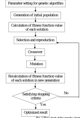
solutions but can replacethem if better solutions are obtained in any iteration. The flow chart for the genetic algorithm is shown in Fig. 1.

Fig. 1 Flow chart of the genetic algorithm

The working of GA is now demonstrated by the following example:

2 2 2 2

Maximize Z  x -y + 2xy x y- +xy

for 0

 

x

5, 0



y



5

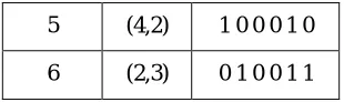
The initial population of solutions, i.e., sets of design variables within the bounding limits is generated at random. InTable 1, column 2contains the randomly generated solutionsand binary coded strings representing them are given in column 3.

Table 1 Initial population for genetic algorithm example

Solution (x, y) String

1 (2,4) 0 1 0 1 0 0

2 (5,1) 1 0 1 0 0 1

3 (2,0) 0 1 0 0 0 0

4 (3,1) 0 1 1 0 0 1

Parameter setting for genetic algorithm

Generation of initial population

Calculation of fitness function value

of each solution

Selection and reproduction

Crossover

Mutation

Recalculation of fitness function value

of each solution in new generation

Satisfying stopping

criteria

5 (4,2) 1 0 0 0 1 0

6 (2,3) 0 1 0 0 1 1

Next, the objective function values, Z,corresponding to these solutions are calculated, given in Table 2. The probability of selection of good solutions is now calculated as:

6

1





i

i i

Z

Z

The probability and cumulative probability for eachsolutionare givenin columns 5 and 6 of in Table 2, respectively.

Table 2 Selection of solutions to generate new generation

Solution (x,y) String

generated f(x,y) Probability

Cumulative probability

Random number

String copied

1 (2,4) 0 1 0 1 0 0 20 0.2817 0.2817 0.7734 1 0 0 0 1 0

2 (5,1) 1 0 1 0 0 1 14 0.1972 0.4789 0.1536 0 1 0 1 0 0

3 (2,0) 0 1 0 0 0 0 4 0.0563 0.5352 0.4123 1 0 1 0 0 1

4 (3,1) 0 1 1 0 0 1 8 0.1127 0.6479 0.9734 0 1 0 0 1 1

5 (4,2) 1 0 0 0 1 0 12 0.1690 0.8169 0.7657 1 0 0 0 1 0

6 (2,3) 0 1 0 0 1 1 13 0.1831 1.0000 0.9342 0 1 0 0 1 1

Using roulette-wheel selection scheme that assigns a probability proportional to the fitness or objective function value, the good solutions are selected. The random numbers corresponding to the probability are shown in seventh column of Table 2. The solutions are copied according to the cumulative probability range in which these random numbers fall.This represents anew population with multiple copies of the good solutions as given in column 7 of theTable 2.

Now, single point crossover operator is used to generate new solutions.Crossover site from where the exchange of bits takes place is selected randomly as shown below.For a random number generated, thecorresponding bit is selected for crossover. In this example, therandom number generated was 0.6529.As it falls in the range of 0.52-0.68, thefourth bit is selected for crossover between parents to generate children.

Fig. 2 Crossover site selection

1 0 0 0 0 0

0 1 0 1 1 0

1 0 0 0 1 0

0 1 0 1 0 0

Parents

_Children

0.00-0.17

Random number range

Fig. 3Parent’s crossover to produce children

The selected crossover site may be same or different for different pairs of parents.

5. Next, the bitwise mutation takes place for this new set of solutions to further explore the search space. A particular bit of the strings is selected for which value is changed from 1 to 0 or vice versa. For the problem considered, it is decided that mutation takes place forthe third bit of the string. A criterionis also setthat mutation operator will be used for a particular string onlyif the random number generated is greater than 0.8. Using this criterion for the problem considered, arandom number is generated for each string representing solutions. The random number generated for fourth and six strings was above 0.8,and hence mutation operator was used for them.

Fig. 4 Bitwise mutation

The final set of solutions after mutation is in Table 3:

Table 3 Final population at the end of one iteration of genetic algorithm

String

generated (x,y) f(x,y)

1 0 0 0 0 0 (4,0) 16

0101 0 0 (2,4) 20

101 0 11 (5,3) 16

0 1 1 0 0 1 (3,1) 8

1 0 0 0 1 1 (4,3) 19

0 1 1 0 1 0 (3,2) 11

Though the maximum value of the objective function for these solutions, i.e., 20 is same as those of the initially generated population of solutions but the average value is increased to 15 from 11.84.Thiscompletesan iteration of GA that improves the

1 0 1 0 1 1

0 1 0 0 0 1

1 0 1 0 0 1

0 1 0 0 1 1

1 0 0 0 1 1

0 1 0 0 1 0

1 0 0 0 1 0

0 1 0 0 1 1

1 0 0 0 0 0

0 1 0 1 1 0

1 0 0 0 0 0

0 1 0 1 1 0

1 0 1 0 1 1

0 1 1 0 0 1

1 0 1 0 1 1

0 1 0 0 0 1

1 0 0 0 1 1

0 1 1 0 1 0

1 0 0 0 1 1

maximum and average value of the objective function by using genetic operators. This final set of solutions is used as the initial population for the next iteration.Thus, the parameters required to start GA are: population size indicating number of solutions, number of iterations necessary for the termination criterion, crossover probability, mutation probability, number of design variables, range of design variables and string length for binary version.The limitations of GA are that (1) it requires a large amount of computational work and (2) there is no absolute guarantee that a global solution is obtained. These drawbacks may be overcome by using parallel computers and by executing the algorithm several times or allowing it to run longer (Arora, 1989).These drawbacks motivate us to explore other optimization techniques which are suitable for the mechanism design.

H. Teaching-learning-based Optimization Algorithm

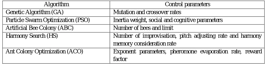
The teaching-learning-based optimization (TLBO) algorithm is also a population-basedoptimization method thatconverges to the optimum solution by using a population of the solutions. TLBO is known as a parameter-less optimization algorithm as no algorithm-specific parameters are required to be handled to implement it (Rao and Savsani, 2012). Whereas, in GA, the parameters like crossover rate and mutation rate are to be optimally controlled to solve the optimization problem.Thus, the main limitation of the available evolutionary optimization algorithms including GA is the optimum setting or tuning of the algorithm-specific parameters for the proper working of the algorithms. The improper selection of these control parameters may results in local optimum solution alongwith therequirement of more computational efforts. The difficulty further increases with the modification and hybridization of the algorithms. The hybridization of the algorithms means combining the properties of the different optimization algorithms to improve the effectiveness of the algorithm. The modification in a particular optimization method suits well to a specific problem and may not work for the other applications. Furthermore, for any modification in an optimization algorithm, it is required to check that algorithm for a wide variety of the problems before drawing any general conclusions for the modifications incorporated.The control parameters required by the popular evolutionary and swarm intelligence based optimization algorithms other than population size and numbers of iterations are listed in Table 4 (Rao and Savsani, 2012).

Table 4Controlling parameters for different evolutionary optimization algorithms

Algorithm Control parameters

Genetic Algorithm (GA) Mutation and crossover rates

Particle Swarm Optimization (PSO) Inertia weight, social and cognitive parameters

Artificial Bee Colony (ABC) Number of bees and limit

Harmony Search (HS) Number of improvisation, pitch adjusting rate and harmony

memory consideration rate

Ant Colony Optimization (ACO) Exponent parameters, pheromone evaporation rate, reward factor

In TLBO, a group of learners is considered as the population and different subjects offered to the learners is considered as design variables. The learners’ result is analogous to the objective function value of the optimization problem. TLBO works in two successive phases in each iteration explainedas follows.

1) Teacher phase –learning from the teacher

In this phase, the learners learn from the teacher. The teacher should be the most experienced and knowledgeable person for a subject. Thus, the learner with the best result is identified as the teacher. The teacher increases the mean result of the population and outcome depends on the quality of teacher as well as learners. In this phase, subject marks of all learners are updated on the basis of subject marks of the learner with the best solution, i.e., teacher.

Each learner’s results corresponding to initial and updated marks are compared,and the subject marks corresponding to the better result are kept for the learner who becomes part of thenew population. The Teacher phase ends with thecreation of new population. This population of the Teacher phase is treated as the initial population in the second phase, i.e., Learner phase of the algorithm. 2) Learner phase :learning through interaction

In this phase, the learners gain knowledge through discussion and interaction among themselves. The Learner phase starts with the final population obtained in the Teacher phase. To improve the marks, each learner interacts randomly with at least one other learner in the population. The learner improves his/her subject marks if another learner has more marks in corresponding subjects.

The flow chart for the TLBO algorithm is shown in Fig. 5. The various parameters of TLBO algorithmare defined as: p = Population size, i.e., number of learners

s = Design variables, i.e., subjects offered to learners LLk,ULk= Lower and upper limits for kth subject marks

n = Number of iterations

i = ith Iteration, i.e., a teaching-learning cycle Zj= Objective function value ofjth learner

Mk= Mean of marks kth subject forthe population

Bk= Marks of kth subject of best learner whose objective function value, Zj,

is minimum

R= random number

3) Algorithm begin: % Initialization of marks for each subject for thewhole population forj=1,…,p

fork=1,…,s

% Marks of kth subject of jth learner,

m







UL

LL

R



LL

m









(1)

end end

% Mean marks of kth subject for the population

p

m

M





% Updating the subject marks of all learners fori=1,…,n







B

M

R



m

m









(3)

% Compute and compare the updated value of

Z

Z

If

Z

Z

% Updating marks 0 2 jk i jk,

m

m



m

m



% End of Teacher phase % Start of Learner phase

% Result comparison of two learnersj and l in population,

m

forj=1,…,l,…,p and if l≠ j

If

Z

Z

fork=1,…,s







m

m

R



m

m









else







m

m

R



m

m









894

end

% Comparison of updated value of

Z

Z

If

Z

Z

% Updating marks 2 4

jk i jk,

m

m



else 3 4

jk i jk,

m

m



% Conditions to check limits of subject marks





i

jk,

m

LL

m



max

,





i

jk,

m

UL

m



min

,

end

% End of ith iteration

4) Algorithm end: The parameter R represents a random number within arange of 0 and 1 which may have adifferent value for different equations. The population obtained at the end of Learner phase is treated as the final population of the current iteration, and this is used as the initial population for Teacher phase in the next iteration. From the final population of the last iteration, the best solution is obtained as the optimum solution. To handle the constraints, the heuristic constrained handling method (Deb, 2000) is used in which the tournament selection operator selects and compares two solutions by following specific heuristic rules. These rules are implemented at the end of the Teacher phase and the Learner phase.

The example solved in the previous section is used now to demonstrate the working of TLBO algorithm.

2 2 2 2

Minimize Z x -y + 2xy x y- +xy

for 0

 

x

5, 0



y



5

Let the population size is the same as used in genetic algorithm.

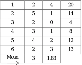
a) At first in Teacher phase, the marks for each subject for initial population of six learners, i.e., sets of design variables within the bounding limits are generated at random using Eq. (1). In Table 5, columns 2 and 3 contain the randomly generated marks of two subjects, x and y. Column 4 presents the value of objective function, i.e., the result of learners.

b) The mean of marks in each subject for all learners is calculated using Eq. (2) and shown in the last row of the Table 5.

Initialize marks for each subject (

k

=1,2,….

s

) for whole population (

j

=1,2,….

p

)







UL

LL

R



LL

m









Calculate mean marks of

k

th subject for the population

m

p

Fig. 5 Flow chart of the TLBO algorithm

Table 5 Initial population generation for TLBO example

Learner Subjects Result

Z

1 2 4 20

2 5 1 14

3 2 0 4

4 3 1 8

5 4 2 12

6 2 3 13

Mean _{3 1.83}

c) The learner with thebest result, i.e., minimum value of Zis treated as the teacher. Hence, learner 3 becomes teacherand the subject marks of all learners are now updated on the basis of teacher’s marks using Eq. (3). The updated values of subject marks and result of all learners are shown in the Table 6.

Table 6 Modified populationin Teacher phase

Learner

Subjects

x y Result

Z

1 1.1853 2.9992 5.9680

2 4.8730 0.7116 15.7448

3 1.0866 -0.2597 0.9288

4 2.3676 0.6867 5.6528

5 3.9025 0.7079 11.4282

6 1.7215 2.9417 10.6175

d) Now, the updated result of each learner is compared with his/her previous result, and the better value is kept along with the respective subject marks as the new set of solutions, given in Table 7. This completes the Teacher phase of the TLBO algorithm.

e) In Learner phase, each learner’s result is compared with at least one another learner randomly chosen in the population and subject marks are updated accordingly using Eq. (4) or Eq. (5).

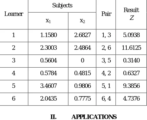
f) Next, the updated result of each learner is compared with his/her previous result, and the better value is kept along with the respective subject marks as the new set of solutions. This completes the Learner phase of the TLBO algorithm (Table 8).

Table 7 Modified population at the end of Teacher phase

Learner Subjects

x y Result

Z

1 1.1853 2.9992 5.9680

2 5 1 14

3 1.0866 -0.2597 0.9288

4 2.3676 0.6867 5.6528

5 3.9025 0.7079 11.4282

6 1.7215 2.9417 10.6175

g) Finally, the subject marks obtained are checked to confirm within the bounding limits (Table 9).

Table 8 Modified population in Learner phase

Learner

Subjects

Pair Result

Z

x1 x2

1 1.1580 2.6827 1, 3 5.0938

2 2.3003 2.4864 2, 6 11.6125

3 0.5604 -0.5268 3, 5 -0.2329

4 0.5784 0.4815 4, 2 0.6327

5 3.4607 0.9806 5, 1 9.3856

6 2.0435 0.7775 6, 4 4.7376

Table 3.9 Modified population at the end of Learner phase

Learner

Subjects

Pair Result Z

x1 x2

1 1.1580 2.6827 1, 3 5.0938

2 2.3003 2.4864 2, 6 11.6125

3 0.5604 0 3, 5 0.3140

4 0.5784 0.4815 4, 2 0.6327

5 3.4607 0.9806 5, 1 9.3856

6 2.0435 0.7775 6, 4 4.7376

II. APPLICATIONS

Guo et al. (2000) used GA to solve an optimization problem formulated to balance planar mechanism based on three different approaches – (1) mass redistribution, (2) counterweight addition and (3) mixed mass redistribution. The results obtained using genetic algorithm was found better as compared to the traditional nonlinear optimization technique. A hybrid genetic algorithm (HGA) was used by Yang et al. (2005) for the vibration optimum design for the low-pressure steam-turbine rotor of a 1007-MW nuclear power plant. This hybridized algorithm (HGA) combines a genetic algorithm and a local concentration search algorithm using a modified simplex method. The shaft diameter, bearing length and clearance were chosen as the design variables to minimize the resonance response of the second occurring mode in the excessive vibration. It was proved that the HGA reduces the excessive response at the critical speed and also improves the stability.Erkaya and Uzmay (2009, 2013) used GA to investigate the effect of joint clearances on the dynamic properties of the planar mechanism. Using the concepts of physical pendulum and inertia counterweights, the optimization problem formulated for balancing of a planar four-bar mechanism is solved using multiobjective particle swarm optimization, and non-dominated sorting genetic algorithm II (Farmani et al., 2011).

III. CONCLUSIONS

This paper discusses various classical and evolutionary optimization techniques followed by the terms defining their working. The popular evolutionary optimization techniques, genetic algorithm (GA), and teaching-learning-based optimization (TLBO) algorithm are presented in details and explained by solving a numerical example. The application of these optimization techniques in different areas including the mechanical design is also highlighted.

REFERENCES

[1] Arora, J.S., 1989, Introduction to optimum design, McGraw-Hill Book Company, Singapore.Deb, K., 2000, “An Efficient Constraint Handling Method for Genetic Algorithm”, Computer Methods in Applied Mechanics andvEngineering, 186, pp. 311-336.

[2] Deb, K., 2010, Optimization for Engineering Design – Algorithms and examples, PHI Learning Private Limited, New Delhi.

[3] Erkaya, S., 2013, “Investigation of Balancing Problem For A Planar Mechanism Using Genetic Algorithm”, Journal of Mechanical Science and Technology, 27 (7), pp. 2153-2160.

[4] Erkaya, S., and Uzmay, I., 2009, “Investigation on Effect of Joint Clearance on Dynamics of Four-bar Mechanism”, Nonlinear Dynamics, 58, pp. 179-198. [5] Farmani, M.R., Jaamialahmadi, A., and Babaie, M., 2011, “Multiobjective Optimization For Force and Moment Balance of A Four-bar Linkage Using

Evolutionary Algorithms”, Journal of Mechanical Science and Technology, 25 (12), pp. 2971-2977.

[6] Gao, Y., Shi, L., and Yao P., 2000, “Study on Multi-Objective Genetic Algorithm”, Proc. of 3rd _{World Congress on Intelligent Control and Automation, June}

28-July 2, Hefei, P R China.

[7] Guo, G., Morita, N., and Torii, T., 2000, “Optimum Dynamic Design of Planar Linkage Using Genetic Algorithms”, JSME International Journal Series C, 43 (2), pp. 372-377.

[8] Holland, J.H., 1992, Adaptation in Natural and Artificial Systems, An Introductory Analysis with Applications to Biology, Control, and Artificial Intelligence, The MIT Press, USA.

[9] Mallipeddi, R., and Suganthan, P.N., 2010, “Ensemble of Constraint Handling Techniques”, IEEE Transactions of Evolutionary Computation, 14, pp. 561–579 [10] Mariappan, J., and Krishnamurty, S., 1996, “A Generalised Exact Gradient Method for Mechanism Synthesis”, Mechanism and Machine Theory, 31(4), pp.

413-421.

[11] Marler, R.T., and Arora, J.S., 2004, “Survey of Multi-Objective Optimization Methods for Engineering”, Structural and Multidisciplinary Optimization, 26 (6), pp. 369-395

[12] Marler, R.T., and Arora, J.S., 2010, “The Weighted Sum Method for Multi-Objective Optimization: New Insights”, Structural and Multidisciplinary Optimization, 41, pp. 853-862.

[13] Montes, E., Coello, C.A.C., 2005, “A Simple Multi-Membered Evolution Strategy to Solve Constrained Optimization Problems”, IEEE Transactions of Evolutionary Computation, 9(1), pp. 1-17

[14] Rao, R.V., and Savsani, V.J., 2012, Mechanical Design Optimization Using Advanced Optimization Techniques, Springer-Verlag London, UK.

[15] Rao, R.V., and Waghmare, G.G., 2014, “A Comparative Study of a Teaching–Learning-Based Optimization Algorithm on Multi-Objective Unconstrained and Constrained Functions”, Journal of King Saud University – Computer and Information Sciences, 26, pp. 332–346

[16] Rao, R.V., Savsani, V.J., and Vakharia, D.P., 2011, “Teaching-Learning-Based Optimization: A Novel Method for Constrained Mechanical Design Optimization Problems”, Computer-Aided Design, 43, pp. 303-315

[17] Rao, R.V., and Patel, V., 2013, “Multi-Objective Optimization of Heat Exchangers Using A Modified Teaching-Learning-Based Optimization Algorithm”, Applied Mathematical Modelling, 37, pp. 1147–1162

[18] Rao, R.V., and Patel, V., 2013, “Multi-Objective Optimization of Two Stage Thermoelectric Cooler Using A Modified Teaching–Learning-Based Optimization Algorithm”, Engineering Applications of Artificial Intelligence, 26, pp. 430–445

[19] Runarsson, T.P., and Yao, X., 2005, “Search Biases In Constrained Evolutionary Optimization”, IEEE Transactions on Systems, Man and Cybernatics, 35, pp. 233–243

[20] Takahama, T., and Sakai, S., 2006, “Constrained Optimization by the Constrained Differential Evolution with Gradient-Based Mutation and Feasible Elites”, Proceedings of IEEE congress on evolutionary computation, Vancouver, BC, Canada, pp. 1–8

[21] Tessema, B., and Yen, G., 2006, “A Self Adaptive Penalty Function Based Algorithm for Constrained Optimization”, Proceedings of IEEE congress on evolutionary computation, Vancouver, BC, Canada, pp. 246–253.