Computational Fluid Dynamics Imitations and
Validation throughout Test Data of a Pipe with
Angle of Inclinations
Tharoon T1
1
Project Assistant, Department of Mechanical Engineering,Coimbatore Institute of Engineering and Technology,Coimbatore-641109, Tamilnadu, India.
Abstract: The main intent of this research work is to find out the contribution of angle of inclination on flow of fluid in a pipe and to study comparative analysis of various viscous model. A comparative analysis is done containing the data of test of a pipe with inclination such as 0o, 30o, 45o, 60o and 90o to determine the competence of the laminar and various turbulent model such as Standard K-epsilon, RNG K-epsilon and K-Omega in CFD. Models of pipe with inclination 0o, 30o, 45o, 60o and 90o are created in ANSYS SPACECLAIM, meshing is done with help of grid sensitivity analysis and the analysis is carried out in ANSYS FLUENT. In order to determine the validity of the models developed and simulation results and the outlet pressure of the fluid in a pipe with inclination 0o, 30o, 45o, 60o and 90o have been gathered and selected laminar and various pertinent turbulent model such as Standard K-epsilon, RNG K-epsilon and K-Omega which generated results close to data of test. It can be noted that the contribution of the angle of inclination of the pipe is not significant on the pressure drop of the fluid flow in the pipe and the experimental outlet pressure of the fluid in the pipe with 0o, 30o, 45o, 60o and 90o is matched with K Omega model results. This research work confirms that the numerical analysis validation and created models useful in the design and performance of the pipe.
Keywords: pipe inclination, model, CFD, viscous.
I. INTRODUCTION
Pipe communications are very important in industries because of the fluids is transported from one place to another place through pipe networks. The pipe flow analysis is very essential in engineering field. Several engineering problems deals with flow analysis. The analysis of flow is very essential because of intermissive engineering applications. The viscous effects and other effects are takes place in flow of fluid in a pipe.
These effects are identified to be acceptable to laminar and turbulent flow conditions. The computational fluid dynamics (CFD) codes are FLUENT, CFX, STAR CFD, FIDAP, ADINA, CFD2000 and PHOENICS in the design and analysis of flow problems [23] that require huge amounts of computer power, memory and computational time [4, 5]. In order to become a summation of all process of design, the CFD developmental activities are progressing hastily.
Due to lack of universally applicable turbulent models, there is a need to examine the adequacy of CFD simulations with test data [6]. Hence, validation through testing is essential for all kind of design and numerical simulations of flow analysis. [7-16]. In order to scrutinize the competence of the models of turbulent in computational fluid dynamics (CFD) codes, a contrastive study is done in
this research paper containing the test data of a pipe with inclination 0o, 30o, 45o, 60o and 90o. ANSYS (FLUENT) is used for done
the flow analysis for the indicated boundary conditions.
The outlet pressure of the fluid in the pipe with inclination 0o, 30o, 45o, 60o and 90o have been obtained and compared with the
measured pressure of the fluid to trace the pertinent turbulent model which generated results nearer to the measured values. Contour plots of pressure are obtainable for the specified boundary conditions. The evaluations of outlet pressure are matching well with measured values.
The numerical analysis is validated by the experiment and accomplished models through comparison of data in the study will be
useful in the design of pipe with inclination 0o, 30o, 45o, 60o and 90o. Literature surveys from various works explored that pipe
II. METHODOLOGY A. Problem Description
Pipe lines are used in industry and it plays an important role in flow of fluid. In this study a pipe is considered with inclinations such
as 0o, 30o, 45o, 60o and 90o. The main objective is to find out whether inclination affect the fluid flow or not and which inclination
gives low pressure drop. Here, the nature of the flow is considered that means the problem can be divided into four cases. Case 1: laminar flow, Case 2: K Epsilon Standard, Case 3: K Epsilon RNG, Case 4: K Omega
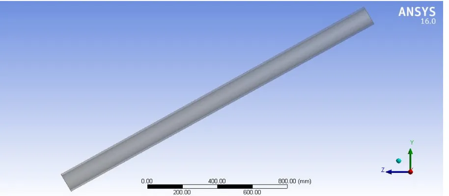
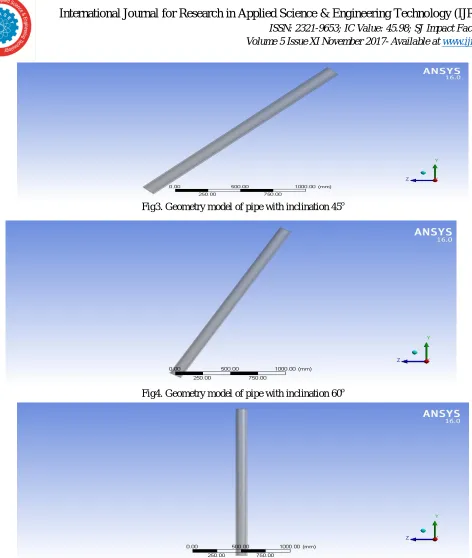
B. Geometry
The geometry of pipe with inclinations such as 0o, 30o, 45o, 60o and 90o was created on ANSYS SPACECLAIM to study the
pressure drop of the fluid when flow enters a pipe with inclinations such as 0o, 30o, 45o, 60o and 90o. The fluid domain is captured in
the pipe with inclinations such as 0o, 30o, 45o, 60o and 90o in SPACECLAIM. The diameter, length and thickness of the pipe is
[image:3.612.78.534.237.492.2]50mm, 2m and 10mm respectively. The geometry models are shown from the figure 1 to 5.
Fig 1. Geometry model of pipe with inclination 0o
[image:3.612.80.537.521.721.2]Fig3. Geometry model of pipe with inclination 45o
[image:4.612.63.535.15.573.2]Fig4. Geometry model of pipe with inclination 60o
Fig 5. Geometry model of pipe with inclination 90o
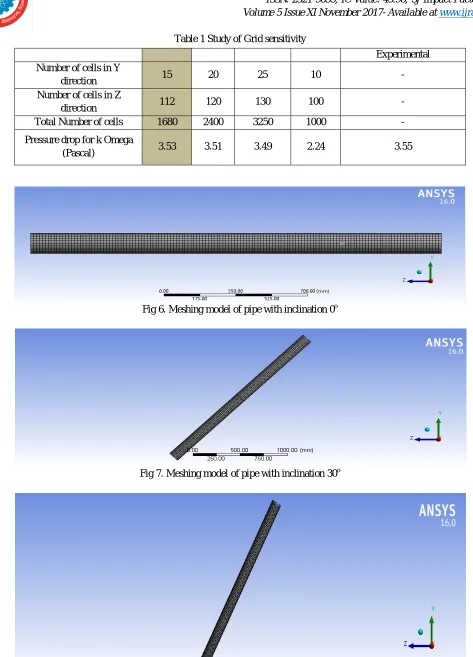
C. Meshing
Table 1 Study of Grid sensitivity
[image:5.612.66.539.44.701.2]Fig 6. Meshing model of pipe with inclination 0o
[image:5.612.94.535.539.721.2]Fig 7. Meshing model of pipe with inclination 30o
Fig 8. Meshing model of pipe with inclination 45o
Experimental Number of cells in Y
direction 15 20 25 10 -
Number of cells in Z
direction 112 120 130 100 -
Total Number of cells 1680 2400 3250 1000 -
Pressure drop for k Omega
Fig 9. Meshing model of pipe with inclination 60o
Fig 10. Meshing model of pipe with inclination 90o
D. Boundary Conditions
For the inlet the velocities of water must be given. The velocities of water at inlet was given as 0.1m/s. At the outlet since the value of pressure was unknown, outflow boundary condition was given for the outlet. The same boundary condition is used for all cases.
E. Simulation
Simulation was performed on the pipe with inclinations such as 0o, 30o, 45o, 60o and 90o generated and applying mentioned
boundary conditions. Simulation was performed for fluid domain on ANSYS FLUENT. A comparative work is done on laminar model and various turbulent models such as Standard K-epsilon, RNG K-epsilon and K-Omega to determine the deviation of pressure of the fluid along the length of pipe and angle of inclination. The pressure velocity coupling affirms SIMPLE algorithm is
used as method of solution. The solution convergence is limited by fitting the residual of relative is 10-6 for all cases.
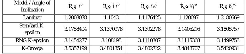
III. RESULTS AND DISCUSSION A. Effect of angle of inclination on pressure drop
The pipe with inclinations such as 0o, 30o, 45o, 60o and 90o is analysed with the help of four models such as laminar model Standard
K-epsilon, RNG K-epsilon and K-Omega. The pressure drop is calculated for each case and it is tabulated in the table 2. From the table we can understand that the influence of angle of inclination of the pipe on pressure drop is not significant. The angle of inclination of the pipe is contributed on pressure drop of the pipe ranges from 1% to 2% deviated among all angle of inclinations such as 0o, 30o, 45o, 60o and 90o
Table 2. Pressure drop for various angle of inclination and turbulence model Model / Angle of
Inclination Ɵ = 0
o
Ɵ = 30o Ɵ = 45o Ɵ = 60o Ɵ = 90o
Laminar 1.2008078 1.1043 1.1176425 1.120097 1.2180669
Standard
K-epsilon 3.1758494 3.1370978 3.1392278 3.1405216 3.1805757
RNG K-epsilon 3.1454277 3.108198 3.1110307 3.1115368 3.1499753
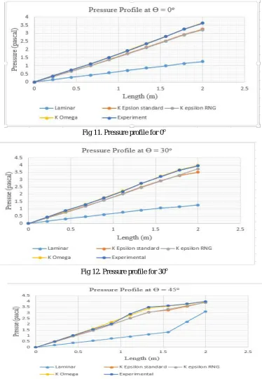
[image:6.612.71.540.619.722.2]B. Comparative study
In this study for all cases the pressure drop varies with respect angle of inclination and laminar model and various turbulent model
such as Standard K-epsilon, RNG K-epsilon and K-Omega. The pressure profile for various angle of inclination (0o, 30o, 45o, 60o
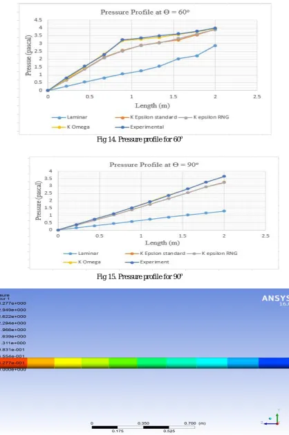
and 90o) is as shown in from figure 11 to 15. By observing the pressure profile for various angle of inclination we can see that
among four models such as laminar, Standard K-epsilon, RNG K-epsilon and K-Omega, the experimental outlet pressure of the
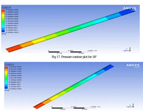
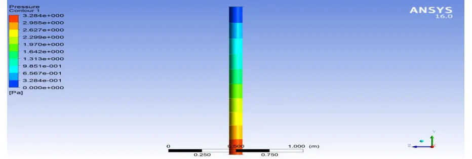
fluid in the pipe with inclinations 0o, 30o, 45o, 60o and 90o is matched with K Omega model results. So the pressure contour plot for
[image:7.612.129.503.172.712.2]K Omega model is shon in the figure 16 to 20.
Fig 11. Pressure profile for 0o
Fig 12. Pressure profile for 30o
Fig 14. Pressure profile for 60o
[image:8.612.128.498.86.272.2]Fig 15. Pressure profile for 90o
[image:8.612.80.541.467.708.2]Fig 17. Pressure contour plot for 30o
Fig 18. Pressure contour plot for 45o
Fig 20. Pressure contour plot for 90o
IV. CONCLUSION
The paper determines the competence of the laminar model and various turbulent model such as Standard epsilon, RNG
K-epsilon and K-Omega in codes of Computational fluid dynamics through comparison of test results of the pipe with inclinations 0o,
30o, 45o, 60o and 90o. The models of a pipe with inclinations 0o, 30o, 45o, 60o and 90o are created by using ANSYS SPACECLAIM,
meshing is done with help of grid sensitivity analysis and the analysis is carried out in ANSYS FLUENT. The outlet pressure of the
fluid in a pipe with inclination 0o, 30o, 45o, 60o and 90o have been gathered and selected laminar and various pertinent turbulent
model such as Standard K-epsilon, RNG K-epsilon and K-Omega which generated results close to data of test. Pressure distribution is presented for the specified inlet and outlet boundary conditions. The appraisement of outlet pressures are well matched with the simulation results obtained by using K omega model. The influence of angle of inclination of the pipe on pressure drop is not significant. There is no widespread turbulent model. The designer has to select an appropriate model through assessment with data of test. This research work confirms that the numerical analysis validation and created models useful in the design and performance of the pipe.
REFERENCES
[1] Henderson D.,” Experimental and CFD investigation of an ICSSWH at various inclinations”, Renewable and Sustainable Energy Review 11 (2007) 1087– 1116.
[2] Rajesh Khatri,” Laminar flow analysis over a flat plate by Computational fluid dynamics”, International Journal of Advances in Engineering & Technology, May 2012, ISSN: 2231-1963.
[3] Sahu M.,” Developed Laminar Flow In Pipe Using Computational Fluid Dynamics”,7th International R&D Conference on Development and Management of water and Energy Resources, 4-6 Feb.2009, Bhubaneshwar, India.
[4] White, Frank M.,”Viscous Fluid Flow”, International Edition, McGraw-Hill, 1991. [5] Bansal R.K. Fluid mechanics and hydraulic machines. Laxmi publication (p) ltd,(2010).
[6] Abdulwahhaba Mohammed, Injetib N K, Dakhilc Sadoun Fahad “CFD Simulation and flow analysis through a T junction pipe” IJEST, 4(7), 3393-3407,(2012).
[7] Crawford N. M, Cunningham .G and Spedding P. L, “Prediction of Pressure Drop for Turbulent Fluid Flow in 90° Bends,” Proceedings of the Institution of Mechanical Engineers, Vol. 217, No. 3, 2003, pp. 153-155.
[8] Spedding P. L, Benard .E and McNally G. M, “Fluid Flow through 90° Bends,” Developments in Chemical Engineering and Mineral Processing, Vol. 12, No. 1-2, 2004, pp. 107-128.
[9] Keon B.J.Mc, M.V.Zagarola, A.J.Smits, A new friction factor relationship for fully developed pipe flow, J. Fluid Mech. (2005), vol. 538, pp. 429–443. [10] Gyorgy, Pinho, and Maia, 2006. “The effect of corner radius on the energy loss in 90 ̊ tee junction turbulent flows”. Department of civil engineering, Faculty
of Engineering, University of Porto
[11] Romero-Gomez, P., C. K. Ho, and C. Y. Choi. (2008). Mixing at Cross Junctions in Water Distribution Systems – Part I. A Numerical Study, ASCE Journal of Water Resources Planning and Management, 134:3, pp. 284-294.
[12] Lahiouel Y., Haddad A., Chaoui K., ―Evaluation of head losses in fluid Transportation networks Sciences & Technologies B – N°23, juin (2005), pp. 89-94 [13] Ansys, Inc. http://http://www.idac.co.uk/products/downloads/Meshing.pdf
[14] Anand B. Desamala, “CFD Simulation and Validation of Flow Pattern Transition Boundaries during Moderately Viscous Oil-Water Two-Phase Flow through Horizontal Pipeline”, World Academy of Science, Engineering and Technology, 73 2013.
[16] Dlamini M. F., Powell M. S. and Meyer C. J. 2005. A CFD simulation of a single phase hydrocyclone flow field. Journal of the South African Institute of Mining and Metallurgy. 105(10): 711-717.
[17] Versteeg H. K. and Malalalsekera W. 2007. An introduction to computational fluid dynamics: the finite volume method Harlow Prentice Hall.
[18] Breuer. M, Jovicic. N and Mazaev .K, "Comparison of DES, RANS and LES for the separated flow around a flat plate at high incidence" Int. J. Num. Meth. Fluids, Volume 41, pp. 357-388 (2003).
[19] Chernyshev. S. L, Kiselev A.Ph, Kuryachii A.P, “Laminar flow control research at TSAGI: Past and present”, Progress in Aerospace sciences, vol. 47, pp. 169-185 (2011).