Comparative study on optimum DG placement for distribution network

J.J. JAMIAN

1

, M. M. AMAN

2

, M.W. MUSTAFA

1

, G. B. JASMON

2

, H. MOKHLIS

2

, A.H.A. BAKAR

2

UniversitiTeknologi Malaysia (1), University Malaya (2)

Comparative Study on Optimum DG Placement

for Distribution Network

Abstract. With the advent of restructuring in power system and the exponential growth in the load demand, the importance of Distribution Generation (DG) has been increased. The DG is used to reduce the power losses and also to improve the system stability. The non-optimum DG placement and sizing could result in increase power losses and instability of the power system. This paper presents the comparative study for DG allocation techniques based on three different indicators namely Active power VSI (P-VSI), Reactive power VSI (Q-VSI) and Power Losses Reduction (PLR) indicator. The performances of these indicators are also compared for optimal DG output, maximum loss reduction, improvement in voltage profile and improvement in voltage stability. Standard 12-bus and 33-bus radial distribution networks are used as a test system. From the analysis and results, it is found that PLR performance is better than P-VSI and Q-VSI indicators in DG allocation.

Streszczenie. W artykule przedstawiono analizę porównawczą technik alokacji kogeneracji rozproszonej, opartych na trzech wskaźnikach: mocy czynnej falownika, mocy biernej falownika oraz redukcji strat mocy. W warunkach optymalnej pracy dokonano porównania maksymalnej możliwej redukcji strat, jakości profilu napięcia oraz stabilności napięcia wybranych metod. W testach systemów uwzględniono standardową 12 i 33-liniową

sieć dystrybucji energii. Przedstawiono wnioski końcowe analizy. (Badania porównawcze metod optymalizacji rozmieszczenia kogeneracji rozproszonej w sieci dystrybucji energii elektrycznej).

Keywords: DG Placement; Sizing; Voltage Stability; Minimum Power Losses.

Słowa kluczowe: rozmieszczenie kogeneracji rozproszonej, wymiarowanie, stabilność napięcia, minimalne straty mocy.

Introduction

Power utilities are facing major challenges as power demand is growing exponentially. In the last decade from 2000-2010, the electricity consumption has been increased by 38% from 15394.16 TWh to 21325.11TWh [1]. However due to congestion in transmission system and less interest of investors in constructing new transmission lines, the possibility of adding new generation sources to the centralized power generations have been reduced. This has resulted the concept of Distributed Generation or Dispersed Generation (DG). Such networks are referred as active networks while those without DGs are referred as passive networks [2]. Different authors have given different definitions of DGs [3-5]. The International Energy Agency defines DG as a small generating plant connected to a distribution network directly connected to the grid at distribution level voltage [3]. In [4-5], the author defines DG as a method of power generation within the distribution network or nearer to the local demand. The purpose of the DG is mainly to provide active power support to the system. However the DG source or technology could be traditional combustion generator such as diesel reciprocating generator and natural gas-turbine, and non-traditional generator including fuel cell, storage device and renewable energy source such as wind turbine and photovoltaic [6-7].

DG has many benefits which makes it attractive and offers good and immediate solution to the ever growing power demand [8]. DG has many advantages in terms of improved system efficiency stability, economical, environmental and technical benefits [9]. In the last few years, the percentage of DG installations has been increased tremendously. For example in Italy 2006, the total number of DG units were 2631, now in 2009 this number has increased to 74,348 generating units (each with less than 10MW) [10]. UK government is targeting to achieve 15% of energy consumption from renewable energy resources as per 2009 Renewable Energy Directive. This will imply raid growth in DG placement [11].

Even though DG allocation and sizing are relatively new, many approaches have been developed to attain the maximum benefit from DG connection. In [12], the authors have introduced multiple DG allocation technique with the aim of minimizing active power losses in radial distribution network using genetic algorithm. In the same direction, the

author in [13] proposes sizing using a new optimization technique called Artificial Bee Colony (ABC) algorithm to optimally size and allocate the DG for real power minimization. In [14], the author has treated the DG distributed generator (DG) placement a hybrid combination of technical and economical factors. The author has configured the problem as multi-objective and solved using genetic algorithm. The authors in [15] has formulated a DG placement a multi-objective function, consists of voltage profile improvements, reduced system losses and as well as short-circuit level. The results have shown that with considering multiple objectives in the analysis, the DG sizing can improved the power losses value and also increased the reliability and security of network.

Researchers have also used the voltage stability index as an indicator for allocating the DG units. This approach improves the voltage stability as well as reduces the power losses of the network. The decline of voltage stability level could be one of the factors which reduces the system loadability of the distribution system [16]. In [17], the optimal planning of DG for improved voltage stability and loss reduction was proposed. In the same direction, the author in [18] has developed a technique for sizing and allocation based on steady state voltage stability index. The technique has enhanced the voltage stability index and at the same time the power losses reduces.

Thus in literature, researchers have used the maximum power losses reduction and the maximization of system voltage stability as the criteria to allocate the DG in the distribution network. The non-optimum DG allocation and sizing could affect the system negatively, increases the system losses and thus reduces the system efficiency. This paper presents a comparative study for DG allocation among three different indicators based on voltage stability index and network power losses reduction. Newton-Raphson method is used to find the power flow solution. The algorithm for the optimal allocation is tested on 12-bus and 33-bus test systems. Numerical results are presented and discussed, as well conclusions are drawn based on the results obtained.

Indicators for optimal DG placement

distribution network. The indictors are termed as P-VSI indicator, Q-VSI indicator and Power Losses Reduction (PLR) indicators. These mathematical indicators are based on the maximum voltage stability and reduce power losses reduction consideration. The complete derivations of these indicators are given in section 2.1 and 2.2.

P-VSI and Q-VSI indicators:

In [19], the author has developed P-VSI and Q-VSI indicators to predict the network health by assessing the voltage collapse point due to active load power increment (Charging Station). By allocating the DG units at highest VSI value in the system, it could improve the stability of the system as well as the power losses value. The formulation of P-VSI and Q-VSI are derived from well known current flow equation as shown in Fig. 1.

             

Rij + Xij Iij

i j n

[image:2.595.345.504.455.662.2]

V1θ1 V2θ2

Fig. 1: An example of the figure inserted into the text

Let ‘i’ as sending and ‘j’ as receiving indicator, thus the current that flows between bus i to bus j can be written as:

(1)

_

























ij ij j j i i ij

jX

R

V

V

I





(2)                      j j j j * j j ij _V jQ P V S I



Comparing Eqns. (1) and (2), we get:

(3) _{j j}

ij ij j j i j

i

_P

_jQ

jX

R

V

)

(

V

V





























_

_

2

Splitting the equation into real and imaginary parts, will give: Real part:

(4)

V

_i

V

_j

cos



_ij



V

_j2



P

_i

R

_ij



Q

_j

X

_ij Imaginary part:

(5)

V

_i

V

_j

sin



_ij



P

_j

X

_ij



Q

_j

R

_ij

The formulation of P-VSI and Q-VSI is stated below:

a. P-VSI

From the imaginary part Eqn. (5):

(6) ij ij j i ij j j _R sin V V X P

Q  



Substitute equation (6) in (4), we will get:

(7) 0

2 2 _                   

 ij j

ij ij j ij i ij i ij ij

j _R R P

X V cos V sin V R X

V  

It is quadratic equations where the root can be determine by using:

(8)

a

ac

b

b

V

j

2

4

2

_







The term inside the square root must be always greater than ‘0’, thus:

(9) 4 0

2 2                   

 _{ij j}

ij ij ij i ij i ij ij P R R X cos V sin V R X





(10)



4

_



2 2



1

i ij ij ij ij ij ij j

V

cos

R

sin

X

Z

R

P





This inequality is termed here as P-VSI:

(11)





2 2

4

i ij ij ij ij ij ij j

V

cos

R

sin

X

Z

R

P

VSI

P



 





b. Q-VSI

From Eqn. 5, the value of Pj is given by:

(12) ij ij j i ij j j

_X

sin

V

V

R

Q

P







Substitute equation (12) in (4), we get:

(13) 0

2 2 _                   

 _{ij j}

ij ij j ij i ij i ij ij

j _X X Q

R V cos V sin V X R

V  

Solving the discriminate of the quadratic Eqn. 13, the formula for Q-VSI is derived as:

(14)





2 2

4

i ij ij ij ij ij ij j

V

cos

X

sin

R

Z

X

Q

VSI

Q











Here it could be observed that the value of P-VSI and Q-VSI could not be greater than unity. Also, when these values reach the unity value, the system becomes de-stabilized. Q-VSI is expressing the impact of reactive power to voltage collapse while the P-VSI is expressing the impact of real power to the voltage collapse. Even though the reactive power (Q) has significant influence on voltage value but in the case of real power increment, it might cause the system to collapse too.

(a)

(b)

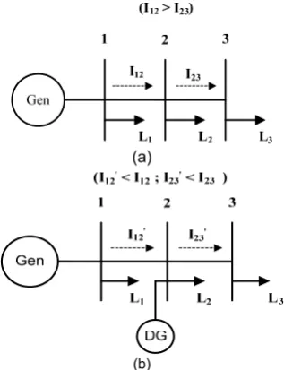
Fig. 2: Losses Reduction due to DG Placement (a) Without DG (b) With DG

PLR Indicator:

[image:2.595.53.290.568.718.2]

(15)

P

_losses





_in_1

I

_i 2

R

_i

[image:3.595.313.537.72.487.2]

where n = number of branches

Fig. 2, shows the situation of the radial network before and after DG integration.

From Fig. 2, it could be observed that the line current between buses 1 to bus 2 is reduced after the DG connection. Therefore, the total power losses in the network also have reduced considerably due to DG placement. The new formulation could be made to show the effect of DG placement in total power loss computation of the network.

(16)

P

_lossesnew





n_i1

I

_inew2

R

_i (17)

P

_lossesnew





n_i1

(

I

_i



JI

_DG

)

2

R

_i

(18) n _i

i i i i DG i DG new

losses I R JI I R J.I R

P _ 



_1 2 ₂  2

where J=1 for feeder that connected to the DG, else J=0. From the equation, the PLR value that can be obtained if the DG is connected at bus ‘i’ is:

(19)

PLR

_i



P

_lossesnew



P

_losses (20)

PLR

_i







n_i1

(

2

JI

_i

I

_DG



JI

_DG2

)

R

_i

The bus that gives maximum negative value of PLR is chosen as the optimal location of DG. Since the formula contained the IDG parameter, it can be determined by

differentiating the PLR formulation with respect to IDG and

set it equal to zero. The optimal DG size also obtained from this IDG value as shown in (22). By using (20) – (22), the

optimal location and size of DG can be obtained.

(21)





 





_n

i i n

i ai i DGi

R

R

I

I

1 1

(22)

P

_DGi



I

_DG

.

V

_i

Flow Chart for Optimum DG Placement:

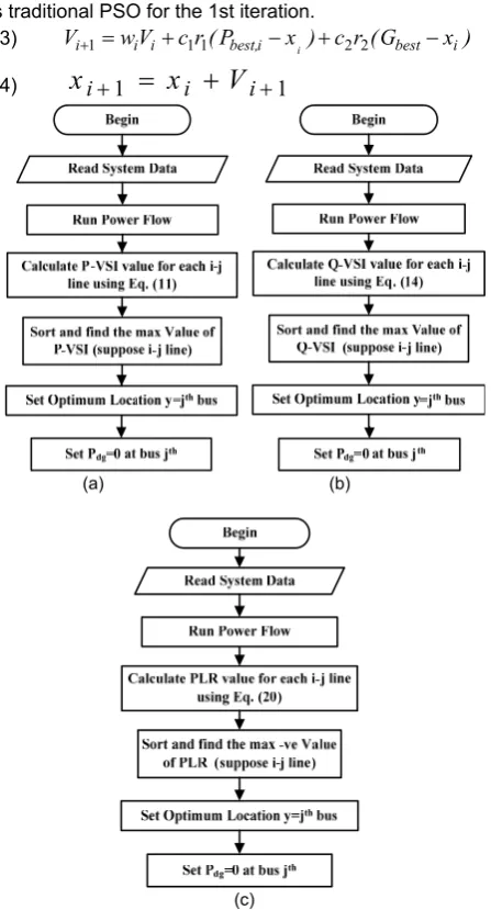
From the above three indicators the optimum DG placement is decided. The flow chart for optimum DG location is shown in Fig. 3.

The application of proposed algorithm on test system will be done in future sections.

Optimum DG sizing based on Rank Evolutionary Particle Swarm Optimization (REPSO)

To get the optimum DG size, optimization algorithm REPSO is employed. It has already been observed that the used of Rank Evolutionary Particle Swarm Optimization (REPSO) gave the fastest computing time and lowest standard deviation value in optimal DG sizing compared to traditional PSO [20]. Fig. 4 shows flow chart of the REPSO in optimization problem of DG sizing.

In this algorithm, “N” number of DG size and set as “x” (particle) are randomized. These random values need to be tested to fulfil all the constraint. The constraints that are used in this study include the generator operation constraint, power balance constraint, injecting power to grid constraint and voltage bus constraint. The “x” values are stored only when all constraints are fulfilled and if otherwise deleted. This step is repeated until “N” number of “x” that obeys the constraints is produced. Next, the global best (Gbest) and local best (Pbest) parameters are determined

based on power losses values that are given by all “x” and

new position (xnew) is obtained using (23) and (24). The step

to finding the Pbest, Gbest and updating the “x” value is similar

as traditional PSO for the 1st iteration.

(23)

V

_i1



w

_i

V

_i



c

1

r

1

(

P

_besti,



x

_i

)



c

2

r

2

(

G

_best



x

_i

)

(24)

x

_i

_

₁



x

_i



V

_i

_

₁

(a) (b)

(c)

Fig. 3: Flow chart for optimum DG placement based on (a) P-VSI (b) Q-VSI (c) PLR

After the new population has generated, the previous and the new population of “x” are pooled together. The concept of ranking, sorting and selection in REPSO is used to determine the best “x” that will be survived in next iteration. Thus, all “x” (previous DG size) and “xnew” (new

DG size) is combined in a one set and are being sorted based on minimum power losses to the highest power losses value. After the sorting process, only the top “N” pool particles are selected as survival particles while the others are terminated. All the survival particles are set as the Pbest

for the next iteration and the top position particle (the lowest power losses) is set as Gbest. Unlike the traditional PSO, two

comparison processes are required to obtain the Pbest and Gbest while in the case of REPSO, all these values are

obtained just after the sorting process is completed. Since all particles in the new iteration are selected as Pbest, the

new velocity equation for updating the position of the particles is become simpler as shown in (25). It is due to the results of subtraction between Pbest and current position

equal to zero.

Therefore, the reduction on comparison process for finding the Pbest and Gbest parameters in each iteration as

[image:4.595.306.541.44.335.2]

well as the process of best particles selection in the REPSO makes the algorithm to reach the convergence faster than traditional PSO and also reduce the total computing time. Thus, the REPSO is used in this analysis to find optimal DG sizing at different location based on indicators results.

Fig. 4: The flow chart for Rank Evolutionary Particle Swarm Optimization Algorithm

Results and Discussion:

The optimum DG location has the impact on the power losses value, voltage stability as well as the voltage profiles of the network. Thus the performance of three indicators for finding the optimal location of DG is studied and an indicator that can give maximum benefit due to the allocation will be considered as the best technique to allocate the DG.

Test Systems:

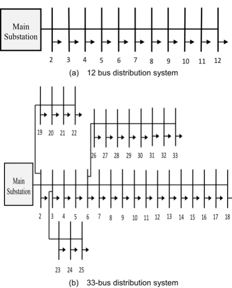
The performance of three indicators is tested on 12-bus and 33-bus radial distribution system, shown in Figs 5(a) and 5(b) respectively and the new DG unit is operated in PV mode.

2 3 4 5 6  7  8  9  10  11  12 

Main Substation

(a) 12 bus distribution system

 

2 3 4 5 6 7 8 9  10  11  12  13  14  15  16  17  18 

19  20  21  22 

26  27  28  29  30  31  32  33 

23  24  25 

Main Substation

(b) 33-bus distribution system

Fig. 5. Single Line Diagram of Test Distribution System

Optimum DG Placement based on P-VSI Q-VSI and PLR Indicators:

The proposed algorithm (shown in Fig.. 3) is applied for optimum DG placement based on P-VSI, Q-VSI and PLR indicators.

[image:4.595.57.289.120.595.2]

Fig. 6 is showing the possible DG allocations for 33-Bus radial distribution networks based on the proposed three indicators.

Fig. 6.The indicators value to determine the optimal location of DG

From Fig. 6, it could be observed that the DG location in case of P-VSI and PLR indicator is same while for Q-indicator, it is differing. Table 1 gives the summary for possible DG placement for 12-bus and 33-bus test systems based on three proposed.

Table 1. Optimal location of DG based on 3 different indicators in distribution network

Test Syst ems

Allocation based on P-VSI

Allocation based on Q-VSI

Allocation based on PLR value

Max P-VSI Value

O Q-VSI Max Value

O Max PLR _Value O

12 bus 0.0369 5 0.1018 8 9.7292 9

33 bus 0.0799 6 0.0674 3 92.127 6

[image:4.595.309.544.456.575.2]

To find the optimal DG location, it is necessary to see the possible impact due to all possible locations on voltage stability and system power losses. The analyses on the DG sizing, power losses and others due to the DG location are discussed in next section.

Optimal DG sizing and Impact of DG allocation to the Power Losses:

[image:5.595.49.292.204.362.2]

From the possible DG locations determined by the three indicators, the optimal DG size is calculated using the REPSO technique. Table 2 summarizes the optimal DG size and corresponding power losses for the given test systems.

Table 2. Optimal DG size based on 3 different indicators in distribution network

Optimal DG location

Power Losses(kW)

Optimal DG Size(MW) 12-Bus Distribution Network

Initial

Condition NA 20.6919 NA

P-VSI based 5 6.2982 0.3386

Q-VSI based 8 3.3141 0.2754

PLR based 9 3.1551 0.2358

33-Bus Distribution Network Initial

Condition NA 203.1854 NA

P-VSI based 6 61.5481 2.4735

Q-VSI based 3 133.8808 3.4604

PLR based 6 61.5481 2.4735

From Table 2, it could be observed that

1. Different DG positions will give the different optimal DG size and power losses.

2. The power losses in the network have reduced considerably after the DG connection regardless the DG location. The power losses improvement that is achieved for the 12 bus distribution system after the DG connection is around 69 to 85 percents and 34 to 69 percents for the 33 bus distribution system.

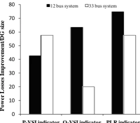
3. The PLR indicator give the optimal DG location either for 12 bus or 33 bus distribution cases in comparison to P-VSI and Q-P-VSI indicators (also shown in Fig. 7).

0 10 20 30 40 50 60 70 80

P-VSI indicator Q-VSI indicator PLR indicator

P

o

w

er

L

oss

es

I

m

p

ro

v

em

en

t/

D

G

s

ize

12 bus system 33 bus system

Fig. 7.The power losses improvement per each MW DG size in the network

Here it should be remembered that different methods exists for finding the weakest bus in the system. Some new methods are quite accurate and the output results matches with the PLR indicators [21].

Impact of DG Location to the Voltage Stability Index and Voltage Profile

On the basis of above results, it has shown that the DG placement based on PLR indicator could give the minimum power losses value with the smallest size of DG units. However, both P-VSI and Q-VSI indicators are formulated based on voltage stability index concept. Thus, the impacts

[image:5.595.329.528.407.735.2]

of all indicators results to the stability index should be analysed too. Therefore, the impacts of DG allocation based on the indicators to the stability index value (P-VSI and Q-VSI) after the DG operated in its optimal value is shown in Table 3.

Table 3. Optimal DG size based on 3 different indicators in distribution network

Indicators Optimum DG _location P-VSI max Q-VSI max

12 Bus Distribution Network

Initial Condition NA 0.036932 0.101790

P-VSI based 5 0.028092 0.095457

Q-VSI based 8 0.026312 0.083993

PLR based 9 0.021068 0.071162

33 Bus Distribution Network

Initial Condition NA 0.079955 0.067365

P-VSI based 6 0.062552 0.049019

Q-VSI based 3 0.077095 0.0647345

PLR based 6 0.062552 0.049019

From Table 3, it could be observed that without any DG unit in the system, the maximum value of P-VSI and Q-VSI in the system are 0.03693 and 0.10179 (for 12 bus system) and 0.07996 and 0.06737 (for 33 bus system) respectively. These maximum VSI value is reducing after the DG connection. However, among all VSI reduction results, the optimal allocation of DG units in the distribution network based on PLR indicators gave the smallest value in both cases (12-bus and 33-bus test system). Here it should be remembered that the smallest value of VSI indicates the most stable system that occurred after the DG allocation. The complete VSI profile for 12-bus system is shown in Figs 8(a) and 8(b) respectively.

0.000 0.005 0.010 0.015 0.020 0.025 0.030 0.035 0.040 0.045

1 2 3 4 5 6 7 8 9 10 11 12

P

‐

VS

I

 

va

lu

e

Bus Number

Without DG P‐VSI based (Bus 5)

Q‐VSI  based (bus 8) PLR  based  (bus 9)

(a) The P-VSI results based on different indicators

0.00 0.02 0.04 0.06 0.08 0.10 0.12

1 2 3 4 5 6 7 8 9 10 11 12

Q

‐

VS

I

 

va

lu

e

Bus Number

Without DG P‐VSI based (Bus 5)

Q‐VSI  based (bus 8) PLR  based  (bus 9)

[image:5.595.100.240.494.617.2]

Furthermore, the allocation of DG unit does not only improve the voltage stability index in the system, but also gave huge impacts to the voltage profile of the system. Figs. 9(a) and 9(b) show the voltage profile of 12 and 33 bus distribution system based on 3 indicators. From the results, the PLR indicators still give the best voltage profile compared to others indicators especially for 12 bus system. With the optimal DG location that given by PLR indicators, all voltage value in 12 bus system is operating higher than 0.99p.u and for the 33 bus system, all the buses have the voltage value higher than 0.95p.u. Thus, the profile after the DG allocation using PLR indicators is better (higher) than the voltage profile that provided by other indicators.

0.85 0.87 0.89 0.91 0.93 0.95 0.97 0.99 1.01

1 2 3 4 5 6 7 8 9 10 11 12

Vo

lt

a

g

e

 

(p

.u

)

Bus Number

Initial (w/o DG) P‐VSI indicator Q‐VSI indicator PLR indicator

(a) Voltage profile for 12 bus distribution system

0.85 0.87 0.89 0.91 0.93 0.95 0.97 0.99 1.01

1 3 5 7 9 11 13 15 17 19 21 23 25 27 29 31 33

Vo

lt

a

g

e

 

(p

.u

)

Bus Number

Initial (w/o DG) P‐VSI indicator Q‐VSI indicator PLR indicator

[image:6.595.58.291.201.516.2]

(b) Voltage profile for 33 bus distribution system

Fig. 9. The comparison of voltage profile in Distribution System

From the voltage profile, the lowest voltage value that occurs in the system can be determined. Table 4 shows the minimum voltage value that exists in the network after the DG allocation. The location of minimum voltage point for 12 bus system is similar for all cases except when DG is located based on PLR indicator. In other words, the minimum voltage value in the system occurs at bus 12 for the system without DG or when DG is located at bus 5 (P-VSI) and bus 8 (Q-(P-VSI). However, when DG is located at bus 9, bus 6 becomes the minimum voltage point.

Table 4. The minimum voltage value in the network after DG allocation

Test System

Initial Network

Allocation based on P-VSI

Allocation based on Q-VSI

Allocation based on

PLR Vmin

value O value Vmin O value Vmin O value Vmin O

12 bus 0.943 12 0.974 12 0.989 12 0.991 6

33 bus 0.910 18 0.963 18 0.929 18 0.963 18

*O= Location where minimum voltage occurred

similar minimum voltage location could be seen for the 33 bus distribution system. Although the location of DG based on Q-VSI and PLR indicators are different, the minimum voltage location is still similar which is at bus 18. After the DG allocation, the minimum voltage value for this network has been improved to 0.9286 for Q-VSI indicator result and 0.9626 for P-VSI and PLR indicators. The overall voltage improvement for this system is around 2 percent to 6 percent.

From the whole analysis, the PLR indicator gave the best results in finding the optimal location for DG unit in the distribution network. With the location given by PLR indicator, the system will have lowest power losses value with minimum DG size, lowest voltage stability index (most stable) and highest minimum voltage value in the system. Therefore, it can be concluded that PLR is one of the best options to be used in determining the optimal location of DG unit.

Conclusion

This paper has presented the comparative study of DG allocations based on existing three indicators (P-VSI and Q-VSI and PLR). These indicators are based on maximizing system voltage stability and power loss reduction. Once the DG allocation has been done using the above three indicators, REPSO optimization method is employed to find the optimal value of the DG with minimum power losses as an objective function for the algorithm.

The proposed algorithm is tested on 12 bus and 33 bus radial distribution system. From the results and discussion, the following points could be concluded.

1. Among the three indicators (P-VSI, Q-VSI, PLR), power loss reduction based indicator (PLR) gives the optimal location of DG with lowest power losses, lowest DG size, highest minimum voltage value in the system, better voltage profile and maximum voltage stability. 2. The others two indicators (P-VSI and Q-VSI) have also

improved the power system performances compared to the initial network without any DG unit. However, due to the location that being found by these 2 indicators for the DG placement is not very suitable, it makes the capability for the REPSO in given a better results for the power losses and others is limited.

3. The optimal DG location based on PLR indicator give superior results in comparison to P-VSI and Q-VSI indicators.

REFERENCES

[1] "BP Global Statistical Review of World Energy 2011."

[2] M. Begovic, et al., "Summary of "System protection and voltage stability"," IEEE Transactions on Power Delivery, 10 (1995), nr 2, 631-638.

[3] M. Khederzadeh and A. Ghorbani, "STATCOM modeling impacts on performance evaluation of distance protection of transmission lines," European Transactions on Electrical Power, 21 (2011), nr 8, 2063-2079.

[4] G. Chicco and P. Mancarella, "Distributed multi-generation: A

comprehensive view," Renewable and Sustainable Energy

Reviews, 13 (2009), nr 3, 535-551.

[5] T. Ackermann, et al., "Distributed generation: a definition,"

Electric Power Systems Research, 57 (2001), nr 3,195-204. [6] S. M. Moghaddas-Tafreshi and E. Mashhour, "Distributed

generation modeling for power flow studies and a three-phase unbalanced power flow solution for radial distribution systems considering distributed generation," Electric Power Systems Research, 79 (2009), nr 4, 680-686.

[7] W. Ouyang, et al., "Distribution network planning method considering distributed generation for peak cutting," Energy Conversion and Management, 51 (2010), nr 12, 2394-2401. [8] P. Kundur, et al., "Definition and classification of power

and definitions," IEEE Transactions on Power Systems, 19 (2004), nr 3, 1387-1401.

[9] P. Crossley, et al., "System protection schemes in power networks: existing installations and ideas for future

development," Seventh International Conference on

Developments in Power System Protection, (2001), 450-453. [10] G. Cau, et al., "Energy and cost analysis of small-size

integrated coal gasification and syngas storage power plants,"

Energy Conversion and Management, 56 (2012), 121-129. [11] ENA, "Energy Networks Association (UK). Available at:

http://2010.energynetworks.org/distributed-generation [accessed on 10-08-2011]." 2010.

[12] S. Larsson and A. Danell, "The black-out in southern Sweden

and eastern Denmark, September 23, 2003," IEEE PES

Conference and Exposition in Power Systems, (2006), 309-313.

[13] M. Ismail and T. K. Rahman, "Estimation of maximum loadability in power systems by using fast voltage stability index (FVSI)," Journal of Power and Engineering Systems, 25 (2005), 181-189.

[14] S. Biswas, et al., "Optimum distributed generation placement with voltage sag effect minimization," Energy Conversion and Management, 53 (2012), nr 1,163-174.

[15] F. Capitanescu, et al., "Optimal power flow computations with constraints limiting the number of control actions," IEEE Bucharestin PowerTech, (2009), 1-8.

[16] B. M. Alshammari, et al., "Power system performance quality indices," European Transactions on Electrical Power, 21 (2011), nr 5, 1704-1710.

[17] R. H. Salim, et al., "Impact of power factor regulation on small-signal stability of power distribution systems with distributed

synchronous generators," European Transactions on

Electrical Power, 21 (2011), nr 7, 1923-1940.

[18] N. G. A. Hemdan and M. Kurrat, "Distributed generation location and capacity effect on voltage stability of distribution networks," Annual IEEE Conference in Student Paper, (2008), 1-5.

[19] J.J. Jamian, et al., "Combined Voltage Stability Index for Charging Station Effect on Distribution Network”, International Review of Electrical Engineering-IREE, 6 (2011), nr 7, 3175-3184.

[20] J. J. Jamian, et al., "Comparative Study on Distributed Generator Sizing Using Three Types of Particle Swarm Optimization," Third International Conference on Intelligent Systems, Modelling and Simulation, (2012), 131-136.

[21] M. M. Aman, et al., "Optimal placement and sizing of a DG based on a new power stability index and line losses,"

International Journal of Electrical Power & Energy Systems,

43 (2012), nr 1, 1296-1304,.

Authors:

J.J. Jamian is a PhD student in Universiti Teknologi Malaysia Email: [email protected]

M. M. Aman is a PhD student in University of Malaya, 50603 Kuala Lumpur, Malaysia.Email: [email protected]

M.W. Mustafa is a Professor in Universiti Teknologi Malaysia. G. B. Jasmon is a Professor in University of Malaya. H. Mokhlis is a Senior Lecturer in University of Malaya. A. H. A. Bakar is a consultant in University of Malaya.

The correspondence address is: