Deposited research article
A draft annotation and overview of the human genome
Fred A. Wright*, William J. Lemon*, Wei D. Zhao*, Russell Sears*, Degen Zhuo*, Jian-Ping Wang*, Hee-Yung Yang, Troy Baer, Don Stredney§, Joe Spitzner, Al Stutz§, Ralf Krahe, and Bo Yuan
Addresses: *Division of Human Cancer Genetics, The Ohio State University, 420 West 12th Avenue, Columbus, Ohio 43210, USA.
LabBook.Com, 6600 Busch Boulevard, Columbus, Ohio 43229, USA. Ohio Supercomputer Center (OSC), 1224 Kinnear Road, Columbus,
Ohio 43212, USA. §Department of Computer and Information Science, The Ohio State University, 2015 Neil Avenue, Columbus, Ohio 43210,
USA.
Correspondence: Bo Yuan. E-mail: [email protected]
comment
reviews
reports
deposited research
interactions
information
refereed research
.deposited research
AS A SERVICE TO THE RESEARCH COMMUNITY, GENOME BIOLOGYPROVIDES A 'PREPRINT' DEPOSITORY TO WHICH ANY PRIMARY RESEARCH CAN BE SUBMITTED AND WHICH ALL INDIVIDUALS CAN ACCESS FREE OF CHARGE. ANY ARTICLE CAN BE SUBMITTED BY AUTHORS, WHO HAVE SOLE RESPONSIBILITY FOR THE ARTICLE'S CONTENT. THE ONLY SCREENING IS TO ENSURE RELEVANCE OF THE PREPRINT TO
GENOME BIOLOGY'S SCOPE AND TO AVOID ABUSIVE, LIBELLOUS OR INDECENT ARTICLES. ARTICLES IN THIS SECTION OF THE JOURNAL HAVE NOTBEEN PEER REVIEWED. EACH PREPRINT HAS A PERMANENT URL, BY WHICH IT CAN BE CITED. RESEARCH SUBMITTED TO THE PREPRINT DEPOSITORY MAY BE SIMULTANEOUSLY OR SUBSEQUENTLY SUBMITTED TO
GENOME BIOLOGYOR ANY OTHER PUBLICATION FOR PEER REVIEW; THE ONLY REQUIREMENT IS AN EXPLICIT CITATION OF, AND LINK TO, THE PREPRINT IN ANY VERSION OF THE ARTICLE THAT IS EVENTUALLY PUBLISHED. IF POSSIBLE, GENOME
BIOLOGYWILL PROVIDE A RECIPROCAL LINK FROM THE PREPRINT TO THE PUBLISHED ARTICLE. Posted: 16 February 2001
Genome Biology 2001, 2(3):preprint0001.1–0001.39
The electronic version of this article is the complete one and can be found online at http://genomebiology.com/2001/2/3/preprint/0001 © BioMed Central Ltd (Print ISSN 1465-6906; Online ISSN 1465-6914)
Received: 9 February 2001
This is the first version of this article to be made available publicly. This article has been submitted to Genome Biologyfor peer review.
A draft annotation and overview of the human genome
1
Fred A. Wright, 1William J. Lemon, 1Wei D. Zhao, 1Russell Sears, 1Degen Zhuo,
1
Jian-Ping Wang, 2Hee-Yung Yang, 4Troy Baer, 3,4Don Stredney, 2Joe Spitzner,
3,4
Al Stutz, 1Ralf Krahe, and 1Bo Yuan
1
Division of Human Cancer Genetics, The Ohio State University, 420 West 12th Avenue, Columbus, Ohio 43210, USA.
2
LabBook.Com, 6600 Busch Boulevard, Columbus, Ohio 43229, USA.
3
Department of Computer and Information Science, The Ohio State University, 2015 Neil Avenue, Columbus, Ohio 43210, USA.
4
Ohio Supercomputer Center (OSC), 1224 Kinnear Road, Columbus, Ohio 43212, USA.
Abstract
The recent draft assembly of the human genome provides a unified basis for describing genomic structure and function. The draft is sufficiently accurate to provide useful annotation, enabling direct observations of previously-inferred biological phenomena. We report a functionally
annotated human gene index placed directly on the genome. The index is based on the integration of public transcript, protein, and mapping information, supplemented with computational
Background
The sequence of the human nuclear genome has been completed in draft form by an international public consortium consisting of 16 sequencing centers and associated computational facilities (http://www.nhgri.gov/HGP). A private commercial version of the genome has also been sequenced and assembled using a whole genome shotgun approach [1]. Many lower organisms have been sequenced to date (http://www.tigr.org/tdb/mdb/mdbcomplete.html), but the 3.2 billion base pair human genome is ~25 times as large as the largest currently finished genomes, Drosophila
at 120 Mb [2] and Arabidopsis at 115 Mb [3].
The current public human sequence is primarily based on ~23,000 accessioned bacterial artificial chromosome (BAC) clones covering 97% of the euchromatic portion of the genome
(http://genome.wustl.edu/gsc/human/Mapping). The sequence of these clones is approximately 93% complete to at least 4x coverage (http://www.ncbi.nlm.nih.gov/genome/seq). Thirty percent of the genome is in finished form, including the entire sequence of chromosomes 21 and 22
(http://www.ncbi.nlm.nih.gov/genome/seq/HsHome.shtml). These clones represent the most complete sequence information available, with overlapping clones positioned on a framework map using restriction fingerprinting. However, reduction to a single consensus sequence permits placement of genes and other chromosomal structures in their proper positional context. Recently, the consortium has distributed a working draft assembly of the entire genome that removes
redundancies, orients sequence fragments and clearly indicates gaps arising from sequencing and assembly. The total assembled length is 3.08 billion bp – about 4% smaller than estimates of genome size based on flow cytometry [4], presumably due to the exclusion of constitutive heterochromatic regions and centromeres. Major gaps (50 kb-200 kb) comprise 16% of the assembly, while minor gaps (100 or fewer bp) and low quality calls comprise 0.5%.
Results
Combine and conquer
Functional annotation of the genome is primarily hampered by the lack of a unified transcript index. Current transcript information still largely consists of anonymous and highly redundant ESTs. The situation is further complicated by extensive splicing variation and elusive expression. To address these problems, the Ensembl consortium relies initially on computational prediction, followed by confirmation with EST/protein alignments
(http://www.ensembl.org/Docs/wiki/html/EnsemblDocs/ScienceDocumentation.html). However, pure computational approaches can give differing results [5], and may miss 20% or more of
emphasize internal consistency and result in limited EST populations that only partially overlap.
The genome sequence serves as a powerful arbiter of the quality of EST evidence, and will enable
consolidation of additional exons into transcriptional units. Thus, we adopt a more inclusive
approach.
Our approach is to combine the major public cDNA, EST and protein databases, resolve
redundancies, and place the resulting exonic sequences uniquely on the genome using the program
Blast. We refer to these genomic segments (technically high-scoring segment pairs,
http://www.ncbi.nlm.nih.gov/BLAST/blast_help.html) as “exons,” although the alignment evidence
awaits future biological confirmation. Splicing evidence was carefully maintained within genomic
clones, and across clones using the fingerprint map. For a given transcript, only the best match to
genomic sequence (using splicing evidence, length and high sequence identity) was preserved,
resulting in a unique location for each exonic unit within each database. We have successfully
applied this approach to integrate UniGene consensus sequences into the human genome draft
(Zhou et al., in press).
To compile a truly unique exonic index, redundancies must also be resolved across
transcript databases. We grouped the databases into ranked categories and ordered them within
categories. Transcripts with known boundary information (using the UTR-DB database) [11] or
full-length cDNAs in the HTDB database [12] were given precedence over other records.
Consensus transcripts were given precedence over individual ESTs because they provide greatly
improved specificity, splicing evidence and transcript integrity. We assembled UniGene-based
human (Zhou et al., in press), mouse, and rat consensus transcripts. Collectively, the databases
represent almost all public information on known genes, transcripts and relevant homologous
sequences. When aligned segments overlapped, only the segments from the highest-ranked
categories were used. After resolution of overlapping exons, a new exonic index of contiguous
spliced components was formed. Each member of this new index inherited the rank of its
highest-ranked exon, in order to facilitate subsequent identification of transcriptional units. Our approach
also ensures that known genes are represented only once in the final gene map.
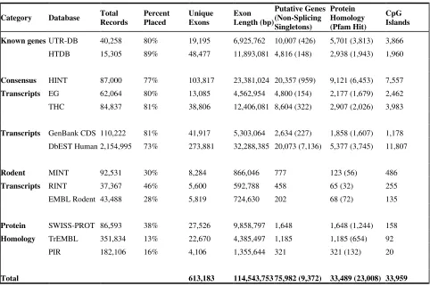
Table 1 describes the identification of exonic sequence via the public databases. Not all
human transcript records could be placed on the genome, reflecting sequence gaps and the draft
quality of the genomic clones. The percentage placement of known genes (80%-89%) suggests that
unsequenced regions will contribute substantial numbers of additional genes. The varying
placement percentages among transcript databases reflect varying sequence quality and differing
transcript lengths. Unique exons are those that have no overlap with those already placed by a
additional placements were possible using protein homology. The percent placement was relatively
low because all proteins from different species were considered, with specificity assured by using
appropriately stringent criteria.
When all of the databases are considered, 613,183 unique exons were placed, including
299,014 in complete open reading frames (ORFs) and 55,860 in partial ORFs. The total putative
exonic lengths add to 106 Mb, or about 4% of the sequenced genome. At least 30-40% of the
known genes or transcript indices contain one or more internal transcripts, suggesting alternative
splicing, internal genes or occasional artifacts (misassembly or genomic contamination). The
prevalence of alternative splicing remains unknown, but may occur frequently [13]. “Sandwiched”
transcripts were merged with their flanking indices, unless both the internal and the flanking
sequences were distinct known genes (<150 apparent internal genes). In addition, we observed a
small number of apparently overlapping genes (~530 on opposite strands) [14].
We assessed three ab initio gene prediction methods by comparing their predicted exons to
the ones identified by transcripts and proteins. Genscan, Grail and Fgene were used across the
genomic clones to identify potential exons. Approximately 70% of the 299,014 exons in ORFs with
either transcript or protein support were identified by at least one of the programs, but a very large
number (847,283) of unconfirmed exons were also identified. A summary of the gene prediction
analyses appears on our web site (http://pandora.med.ohio-state.edu/Annotation). The large
apparent false positive rate implies that pure computational gene prediction is not yet a practical
alternative to experimental evidence.
Transcriptional units
Our consolidated exonic index is of inherent biological interest, but it is desirable to further
identify transcriptional boundaries to create a putative gene index. We employed an approach
designed to minimize fragmentation of exons and provide conservative gene counts (see Methods).
The following criteria were used to identify gene boundaries: (1) known 5′ or 3′ UTR sequences in
UTR-DB; (2) full-length cDNAs in HTDB; (3) exons in partial ORFs as possible boundaries of
coding regions; (4) exons without continuous ORFs as additional UTR sequences; (5) CpG islands;
and (6) gene boundaries predicted by Genscan. Multiple in-frame exons in a continuous ORF were
always considered part of a single gene, an approach that tends to consolidate exons rather than
create spurious additional genes. Additional consolidation resulted from extension of boundaries
for multiple exons not residing in ORFs until occurrence of genomic landmarks described above.
transcripts, and the integrity of ORFs and other genomic landmarks provided by the draft
sequences.
Table 1 lists the number of genes added by each database to the cumulative sum. The total
number of known genes in UTR-DB, HTDB and HINT is 16,673. This compares with 11,191
entries with at least partial functional annotation in UniGene (May ’00 build) and 11,863 entries in
the HUGO Human Gene Nomenclature database (http://www.gene.ucl.ac.uk/nomenclature).
Approximately 48% of the transcriptional units were based on consensus transcripts and 28% based
on individual ESTs. A total of 9,372 transcriptional units were based on singleton transcripts
without splicing evidence, which can result from genomic contamination or other artifacts. A total
of 1,437 units were supported only by rodent transcripts. An additional 3,154 units were identified
based on protein homology. Our approach yields an overall estimate of 75,982 transcriptional units,
with 66,610 supported by multiple transcripts or individual transcripts with splicing evidence. We
observed that 45% of the gene units were associated with CpG islands (defined as 10 kb upstream
or within the gene). For the 6,500 known genes with known 5′ boundaries, the value was 40%. The
average genomic size of each transcriptional unit, including only transcript or protein-based exons,
is ~ 12 kb. In total transcriptional units occupy about 900 Mb, corresponding to approximately 35%
of the sequenced genome.
Gene map
The placement of transcriptional units is not without error, as most genomic clones are unfinished
and the restriction fingerprint map can be subject to misassembly. To resolve placement errors, we
used a relational database to integrate information from several independent maps, including
Genemap ’99, assembled genomic contigs, and fingerprint, radiation hybrid and cytogenetic maps
(See Methods). Placement required a minimum of three concordant criteria. Together, a total of
75,982 transcriptional units were placed on the genome, providing an initial glimpse of a complete
gene map. The map and associated functional annotation (see below) are available at
http://pandora.med.ohio-state.edu/Annotation.
Functional annotation
SWISS-PROT, TrEMBL, PIR and Pfam were used to annotate our unified gene index, because
functional keywords in these databases are standardized [15] (Table 2). We used the classification
schema developed by the International Gene Ontology Consortium to assign each keyword to an
http://pandora.med.ohio-state.edu/Annotation for keyword assignments). Clear functional roles and biological processes
were given priority over other keyword designations. Similarly, protein-based annotation was
performed for HINT consensus transcripts. The transcriptional units resulted in a greater number of
annotations (~23,000) than HINT transcripts (~11,000) because of the increased length of the
included genomic sequence.
The annotation also allows us to assess the protein composition of human vs. other species.
A BlastX result of E < 10-20 was required in cross-species DNA-protein alignments to be considered
homologous. A total of 20,892 human transcriptional units (30% of all units) are homologous to at
least one other species; 5,792 (10%) were conserved across mammals (mouse or rat), Drosophila,
and C. elegans. A total of 1,759 (3%) were conserved across all of these species and yeast. These
values are very consistent with a recent comparative genomic survey [16].
Global tissue expression profiles
During the assembly of UniGene (Zhou et al., in press), we retained the library source for each
EST, via links provided by UniGene to the IMAGE consortium (http://image.llnl.gov). Most of the
2,500 libraries comprising UniGene ESTs were derived from single tissues or embryonic stages,
and we further standardized the library source annotation into 102 categories. Keywords and
derived categories available at http://pandora.med.ohio-state.edu/Annotation. The most highly
represented categories were various types of tumors (15.0% of all ESTs), fetal tissue (10.7%),
embryo (6.2%), infant (5.1%), and testis (4.3%). We reasoned that some genes might exhibit highly
tissue-specific expression, such that most of the ESTs comprising a transcript would be derived
from the tissue. The identified genes are potential candidates for diseases of the involved tissues.
Similar approaches have been used to identify candidate genes for pathologies of the prostate [17]
and retina [18]. We explore here the global nature of tissue/source specificity. The result was
7,459 HINT transcripts highly significant tissue-specificity (11%). Many of these are known genes,
and an examination of the most-specific transcripts revealed clear relationships to the associated
tissue. For example, a search for retina-specific genes revealed that the 10 most significantly
associated with retina include five known genes, all related to retina function. Four are implicated
in retina pathology: GNAT1 and ARR (night blindness), RHO (retinitis pigmentosa), and GUCA1A
(cone dystrophy). Similar results were observed in numerous other tissues, although not as
obviously related to pathology. The results appear especially striking for tissues with substantial
EST representation, including brain, lung, liver, kidney, and testis, suggesting that putative tissue
involvement can be inferred for many anonymous ESTs. Where possible, the tissue expression
the tissue-specific clusters were from embryonic tissue libraries (while such tissue contributed 6.2%
of all UniGene ESTs). This striking result is consistent with the highly regulated and specific
nature of embryonic development [19]. The embryo category is followed by brain (9.7%
brain-specific vs. 3.8% of ESTs) in number of tissue-brain-specific clusters, kidney (5.5% vs. 3.5%), and testis
(6.1% vs. 4.3%). We also examined the locations of the tissue-specific transcripts on the genome,
and found no evidence of regional clustering (see description of regional functional clustering in
Methods).
A global view of the human genome
In keeping with the longstanding clinical importance of cytogenetics, it is important to align
Giemsa-staining G (dark) cytobands vs. R (pale) bands (ISCN 1995) to the assembly [20].
Cytoband boundaries on genomic sequence have been depicted with apparent precision [6, 21] but
in fact are largely unknown. With only a few-fold genomic coverage, the gap sizes in unfinished
sequence are difficult to estimate precisely. Thus, it is preferable to align the cytoband positions to
the fixed assembly rather than the reverse. Such an “assembly-corrected” alignment was performed
using genes/ESTs that have been mapped cytogenetically and also placed on the assembly. This
alignment is approximate, as the resolution of conventional staining techniques and FISH is limited
to 1-3Mb [22].
Density of genomic features
The resulting corrected ideograms and six major genomic features are plotted across the genome in
Figure 1. Unique exons (as determined above), CpG islands, genomic GC content, Alu and LINE1
elements, and minisatellites are plotted as densities (proportion of bases belonging to feature) in 1
Mb intervals. The assembly-corrected ideogram clearly differs from the standard ideogram – e.g.,
in our representation 1p is longer than 1q. This may reflect more complete sequencing on 1p, or
perhaps differing DNA packing densities on the two chromosome arms. Many of the chromosomes
show a suggestive relationship between cytobands and exon density, consistent with the expectation
that R bands are relatively gene rich. A more striking result is the expected positive correlation
among exons, CpG islands, GC content, and minisatellites, which track each other closely on most
chromosomes. Exon density is relatively high on chromosomes known to be gene rich (e.g., 17 and
19) [23], and low on chromosomes 4, 13, X, and Y.
A total of 48,000 CpG islands were found on the assembly using standard criteria [24] (see
Figure 1 legend), with a median length of 336 bp. As sequencing gaps are filled, this number may
CpG-rich region), this number is in close agreement with the estimate of 45,000 obtained by
Antequera and Bird [25] using methylation-sensitive restriction enzymes. The CpG island density
is also in agreement with a report of FISH karyotypes using CpG island probes [26] with
contrasting fluorescent signal in late replicating regions. Extended regions of high CpG island
density, such as the terminus of 1p and 1q21-q22, are apparent in the FISH assay. Short spikes of
CpG islands (e.g., in 3p26 and 3p25 of Figure 1) do not obviously appear in the assay, perhaps
because they are below the resolution of FISH or are part of transcriptionally active regions.
In contrast to exon and CpG island density, GC content shows limited variation – in the
range 35%-55% for most 1 Mb intervals. The overall GC content is 41.1%. This compares with
estimates in the range of 40%-41% based on density gradient centrifugation [27] and flow
cytometry [28].
Consistent with previous reports [29] Alu repeats show an apparent positive correlation with
exon, CpG and GC densities, while LINE1 densities do not show such correlation. Approximately
1.1 million Alu repeats were identified, as expected [30]. However, a total of 758,000 LINE1
repeats were identified – 40% higher than estimates based on a sampling of sequenced regions [30].
Minisatellites of the hypervariable family (20 bp-50 bp repeat size) are dispersed throughout the
genome, but as expected [31] show sharp spikes in subtelomeric regions of most chromosomes.
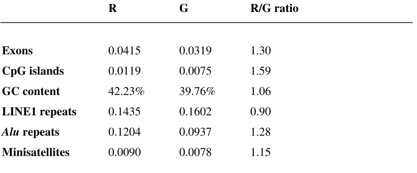
Comparison of cytogenetic bands
We next examined the overall correspondence between cytobands and exonic density and other
genomic features. Table 3 gives the average densities of features in the R bands vs. G bands based
on the assembly-corrected alignment. Genomic intervals residing in R bands were significantly
richer in exons, CpG islands, GC content, Alu repeats and minisatellites than those in G bands. The
reverse is true for LINE1 elements. These observations accord with predictions based on a variety
of indirect methods [32], or a selected set of genes [33], but only now may be investigated directly
using the sequence of the entire genome. The increased exonic density in R bands was fairly
modest (~30%), and may reflect attenuation due to alignment error. In addition, the analysis did not
account for variation in staining intensity in G-bands [20]. However, the results across the
chromosomes were fairly consistent, and the R/G exonic density ratio exceeded 2.0 on two
chromosomes (13 and 21) and was below 1.0 on only one chromosome (Y). The increased density
of CpG islands in R bands was more striking (59%), while GC content was only a few percent
higher (42.2% vs. 39.8% in G bands), again consistent with previous observations [34]. The results
for the cytobands are also reflected in pairwise correlations of the genomic features across 1 Mb
positively correlated. LINE1 elements again differed from other features, showing a negative
correlation with exons, CpG islands, GC content and Alu repeats.
Gene density
We analyzed for each chromosome the exonic sequence as given in Table 1. Figure 2A shows the
density of exonic sequence per chromosome. Chromosomes 19 and 17 are the richest (i.e., densest)
in exonic sequence [23], by factors of 2.04 and 1.62, respectively, compared to the average for the
genome. Chromosomes 4, 13, 21, X and Y are exon-poor. A similar pattern emerges in the density
of transcriptional units across the chromosomes, as shown in figure 2B (Zhou et al., in press).
Reports based on integrated radiation hybrid maps of ESTs [35, 36] indicated that chromosomes 1
and 22 were more gene-rich, but otherwise broadly agree with our results.
An intriguing clinical observation follows from these data and the tissue-specific
observations. It had been noted [32] that the aneuploidies that are compatible with survival until
birth (trisomies 13, 18, and 21, as well as X and Y aneuploidy) appeared to occur in relatively
gene-poor chromosomes. Our data confirm these observations. However, the most obvious models for
the deleterious effects of aneuploidy should instead depend on the total number of genes. In
examining our HINT transcripts we have found that in fact the total number of embryo-specific
transcripts is lowest on these 5 chromosomes (Figure 3). We suggest that trisomy of other
chromosomes may exceed a limit of survivable dosage compensation during development.
Comparisons to genetic and RH maps
A total of 3,628 Genethon markers from the Marshfield map were localized via e-PCR [37] on the
assembly, along with 28,350 Genebridge 4 markers/ESTs and 4,688 Stanford G3 markers appearing
in Genemap ’99. Figure 4 shows the positions of markers on the Chromosome 1 assembly. The
curves are nearly monotonically increasing, showing that the assembly is broadly correct, although
localized orientation errors and outliers remain (plots for all chromosomes appear at
http://pandora.med.ohio-state.edu/Annotation). These plots are immediately useful as they enable
the placement of new markers on genetic maps without the need for mapping experiments. Some of
the variation likely reflects estimation error in the published maps, and the curves are not
completely monotone for finished chromosomes 21 and 22. However, other regions likely reflect
errors in assembly, as the genetic and RH maps agree with each other but disagree with the
assembly (e.g., the 130-148 Mb region is reversed on chromosome 5; a 15 Mb region of Xqter
belongs at Xpter; numerous other isolated reversals and extensive reversals on chromosome 16).
the telomeres, and a low male recombination rate (and thus sex-averaged rate) near the centromere
(~130 Mb). Similar patterns hold for the entire genome. These observations agree with previous
studies which had been limited to comparisons of genetic and RH maps [38], male/female meiotic
ratios [39], or relatively few markers on well-sequenced chromosomes [39]. The plots offer an
interesting perspective on positional cloning efforts. For example, examination of the plots reveals
that the hemochromatosis gene HFE, at 28 Mb on 6p, lies at the edge of a recombination “cold
spot” from 28-40 Mb. This fact complicated efforts to map the gene via linkage disequilibrium
[40]. In contrast, the NIDDM1 gene at 2qter (a region with higher recombination rate) was initially
mapped to a 7 cM region, which fortunately was discovered to be only 1.7 Mb of sequence [41].
The radiation hybrid plots tend to be more linear, which is consistent with the model that
radiation induces chromosomal breakpoints essentially uniformly [42]. However, jumps in the GB4
map occur at the centromere on most chromosomes. This may result from incomplete centromeric
sequencing and assembly, so that a large centromeric gap might not appear as such. Alternatively,
the jumps may reflect statistical difficulties in estimating breakpoint rates across the centromere.
We note that no jump occurs in the G3 map, apparently because the higher radiation intensity
produces insufficient marker pairs in the rescued hybrids that span the centromere. Thus the jump
cannot be accurately estimated and was simply suppressed in the published map
(http://www-shgc.stanford.edu/Mapping). A large unrecognized sequence gap would then appear as a flat region
on G3 plot, which does not occur. An alternative possibility is that the jumps reflect increased
radiation sensitivity at the centromere. This is worthy of additional investigation.
Clusters and compartments
The availability of the full assembly enables a comparison of the entire genome to itself for
evidence of homology arising from duplications or insertions. We emphasize that the genome is
still in draft form, and a complete description of these features will be a large and ongoing scientific
and computational task. We used BlastN [43] to identify intra-chromosomal homology and to
provide an initial look at the genomic landscape. Local duplication is a feature common to all
chromosomes, as evidenced by the near-diagonal runs in dot-matrix plots in which the line of
complete identity has been removed (Figure 5, full page plots for each chromosome at
http://pandora.med.ohio-state.edu/Annotation). These runs vary across the chromosomes, and tend
to be of high sequence identity, indicative of recent origin. More distant duplications also occur,
and include large repetitive regions of high identity on chromosomes 10 and 17. The Y
chromosome shows strong internal sequence similarity, some of which arises from strikingly long
q-terminus of the euchromatic region). Near-duplicate sequences appear through the genome,
producing a “plaid” appearance on many chromosomes. These sequences tend to have lower
sequence similarity (blue in Figure 5), consistent with an ancient origin and accumulated mutations.
As an example of functional duplication, we note that more than 60% of the entire zinc-finger
(ZNF) families are mapped to chromosome 19, restricted to six tandemly duplicated gene clusters
spanning the chromosome. More than one type of ZNF is found within each cluster, presumably
resulting from sequence divergence. A majority of these ZNFs are densely populated within the
22-27 Mb region (see Figure 5). The remaining ZNFs are mapped to 15q21 (bZIP), 7q11 (KRAB),
11q13 (C3HC4), 11q23 (C3HC4), 6p21 (C2H2), 10p11 (KRAB), 10q11 (C2H2), 16p11 (C2H2), 9q22
(C2H2), and 3p21 (C2H2). Regions of high and striking similarity and the list of matching sequences
with protein homology are provided at http://pandora.med.ohio-state.edu/Annotation.
Discussion
Comparison of gene counts
Our count of 66,000-75,000 transcriptional units on the genome is consistent with gene count
estimates [25, 44] that had held sway until recent widely varying estimates [10, 45, 46].
Ewing and Green [10] examined 680 assumed genes on chromosome 22 and found matches to 2%
of a selected set of assembled EST contigs. The sampling approach assumes that the 680 genes
represent 2% of all genes, resulting in an overall count of 34,000. An examination of evolutionarily
conserved regions in known genes on chromosome 22 in humans vs. the fish T. nigorviridis [45]
results in an estimate of ~30,000 genes, assuming a uniform rate of conserved regions per true gene.
These approaches resulted in similar estimates when applied to larger sets of mRNAs or known
genes, and are similar to the current 33,000 genes reported by Ensembl as having Genscan
computational support and EST confirmation. All of these estimates are carefully constructed and
remarkably concordant, and we propose possible explanations for the difference from our results.
The differences do not result entirely from the reliance on transcriptional evidence, as has been
proposed [47].
Our estimate of 854 genes on chromosome 22 is 25% greater than that of Ewing and Green
noted [10], but represents only 1.4% (rather than 2%) of our gene total. It was noted [10] that high
expression on chromosome 22 could result in low gene count estimates by biasing the reference
sample. In addition, known genes may be more highly expressed than unknown genes, which
presumably aided their initial identification and characterization. Our evaluation of EST evidence
supports the existence of both forms of bias. We have found that 5% of Ewing and Green’s original
to chromosome 22. An examination of UniGene transcripts (May ‘00) reveals that the known genes contain a median of 41 entries, while anonymous transcripts contain a median of just two entries.
This is not entirely explained by the greater length of the known gene-like transcripts (having been
correctly assembled as a single unit). In dividing the number of ESTs in the consensus by its
length, we obtain a median of 0.017 entries/bp for known genes and 0.005 entries/bp for anonymous
transcripts. On chromosome 22, the median number of ESTs per anonymous transcripts is three,
which is significantly higher than that among other transcripts on the genome (geometric mean 3.76
vs. 3.11 for other chromosomes, p<0.0001, Wilcoxon rank-sum test). The estimate based on
conserved regions [45] is calibrated using known genes. This approach also introduces bias, as
such genes appear more likely to belong to the evolutionary core proteome. Known genes comprise
22% of all of our transcriptional units, but comprise 71% of our units which are conserved with
rodents, Drosophila and C. elegans. A recent high gene estimate based on transcript evidence [46],
again using chromosome 22, appears to result from less stringent alignment criteria, resulting in
many putative genes.
As genomic annotation proceeds, the number of protein-encoding genes will become
clearer. Our approach seems to rule out artifactual or genomic contamination as the predominant
explanation for transcriptional units with unknown function or protein homology. Ensembl has
recently listed a count of 170,160 ‘confirmed’ exons, while we report 299,014 in complete ORFs
and many more in untranslated regions, suggesting that our approach identifies considerable
additional transcription. We point out that only 58% of known genes exhibit protein homology
(Table 1), and e.g. a large proportion of transcriptional units have not been functionally classified in
Drosophila [2]. We thus propose that most of the unclassified transcriptional units are in fact
coding – the lack of protein homology may reflect difficulty in studying these proteins, or rapid
gene evolution, and some portion is likely to function at the RNA level [48].
Clustering of ontological groups
We examined the locations of all transcriptional units that had been classified according to Gene
Ontology (Table 2) for evidence of regional clustering. We applied a test that corrected for regional
gene density, and found substantial evidence for regional clustering among the transcripts belonging
to the same category (location plots for the top 60 ontological categories at
http://pandora.med.ohio-state.edu/Annotation). Such clustering is pervasive – much of it likely to have arisen from
duplication in which functional units have been preserved.
We also examined the runs of six or more gene units in which the ontological classifications
across the genome appears at http://pandora.med.ohio-state.edu/Annotation. The plot shows clear
evidence of local duplication, while the distant matches (even across chromosomes) are under
investigation in the context of the complete sequence. We have noticed interesting associations
among membrane proteins, ion channels, electron transporters, ATP binding cassettes, and genes
involving metabolism on chromosomes 2, 5, and 7, suggesting that proximity may be important for
regulating functionally coupled genes. This phenomenon is well established in lower organisms
[49]. Similar physical-functional coupling has also been recently reported in yeast [50].
As an additional demonstration of the duplication phenomenon, we considered the
occurrence of Pfam motifs within ORF, with only the best Pfam match retained per ORF (~1,930 of
the 2,011 Pfam categories were represented). Matching successive runs of four or more (that occur
at least three times on the genome) appear on http://pandora.med.ohio-state.edu/Annotation. Many
of the runs occur on the near-diagonal. Most involve four identical Pfam categories in succession,
or a double run of two categories, again pointing to local duplication.
Concluding remarks
The human genome is a capacious resource that will support years of intensive investigation.
The quality of the draft sequence has now reached the point that genetic maps can truly be
integrated into the genome. Analysis at the sequence level shows pervasive local and distant
duplication, much of which preserves function. We have found evidence for a large number of
transcriptional units (65,000-75,000) and performed initial annotation and classification. The
effective study of transcription and protein function requires the compilation of all available
evidence of transcription and protein homology. We have created such a resource to aid in this
effort.
Materials and Methods
Exon identification The June 26, 2000 version of the repeat-masked draft sequences was
downloaded from http://www.ensembl.org and blasted against cDNA and protein sequences by
using the Blast program compiled from the NCBI toolkit (6.1) on a 32-node SGI Linux/Intel
Cluster, with four 550MHz Pentium III Xeons processors and 2GB of RAM on each node. The
following databases were used: Human UTR-DB (EBI) ftp://ftp.ebi.ac.uk/pub/database/UTR (v.
13); HTDB (Baylor University) http://www.hgsc.bcm.tms.edu/HTDB (v. 1); GenBank CDS
(NCBI) ftp://ncbi.nlm.nih.gov/blast/db/nt.Z (only PRI mRNA sequences were used, v. 119); HINT
http://www.phrap.org/est_assembly; THC (TIGR) http://www.tigr.org/tdb/hgi (v. 4.5); dbEST
(NCBI) ftp://ncbi.nlm.nih/blast/db/est_human.Z (v. 119); MINT (Ohio State University)
state.edu/HINT; RINT (Ohio State University)
http://pandora.med.ohio-state.edu/HINT; EMBL Rodent (EMBL) ftp://ftp.ebi.ac.uk/pub/databases/embl/release/rod.dat.gz
(v. 63); SWISS-PROT (EMBL) http://www.ebi.ac.uk/SWISS-PROT (v. 39); TrEMBL (EMBL)
http://www.ebi.ac.uk/SWISS-PROT (v. 14); PIR (MIPS-JIPID) http://pir.georgetown.edu (v. 65);
and Pfam (Sanger Centre) http://www.sanger.ac.uk/Software/Pfam (v. 5.4). The Mouse and Rat
Indices of Non-redundant Transcripts (MINT and RINT) were derived from Mouse and Rat
UniGene (http://ncbi.nlm.nih.gov/unigene) using the same approach we have applied to human
UniGene (Zhou et al., in press). Briefly, chimeric sequences were removed, UniGene transcripts
were assembled into sequence contigs, and links to progenitor records retained.
The genome-wide hit expectation value was set at E<10-25 (BlastN) or E<10-15 (BlastX) to
filter out non-specific high-scoring segment pairs (HSPs). Default parameters of Blast were used.
The Blast report was parsed into field-specific tables using the program MSPcrunch
(ftp://ftp.cgr.ki.se/pub/prog, Version 2.3). The resulting table was processed using a set of Perl
scripts by first retaining only the HSPs that were spliced from the same transcripts on the same
genomic contig. The same process was then applied to the HSPs on the genomic sequences, that
spliced HSPs from the same transcripts were retained followed by the singleton HSPs that were
both longer and higher in sequence identity over their overlapping counterparts, resulting in a
unique placement for each cDNA segment on the genomic sequence.
Prediction of transcriptional units A set of Perl scripts was used to implement the algorithm
described above. Genomic clones were ordered and oriented using the fingerprint map and draft
assembly. Within unfinished clones, sequence contigs were further ordered and oriented according
to Ensembl’s assembly (ftp://ftp.sanger.ac.uk/pub/enembl/data/mysql/contig.txt.table.gz). This
mapping produced the positional context necessary for consolidating fragmented exon units. Where
necessary, small sequencing gaps (100 bp or fewer) were ignored and genomic clones were
considered contiguous except where a large gap was indicated in the draft assembly (>50 kb).
ORFs were determined using the program getorf (http://www.emboss.org).
Gene mapping A relational database was used to integrate multiple largely independent maps for
the genomic clones, where transcripts had been placed. This integration thus results in a transcript
map based on the order and position of genomic clones. Individual sequencing contigs within each
(ftp://ftp.sanger.ac.uk/pub/ensembl/data/mysql/contig.txt.table.gz). The fingerprint
(http://genome.wustl.edu/gsc/human/Mapping, version June 15, 2000), GoldenPath assembly
(Versions June 15 and September 5, 2000), and radiation hybrid maps
(ftp://ncbi.nlm.nih.gov/repository/genemap/Mar1999) were used to place genomic clones into their
chromosomal context. Since a substantial number of the clones in the working draft had not been
physically typed with RH or genetic markers, the program e-PCR [37] and primers collected in the
RHdb (http://corba.ebi.ac.uk/RHdb) and Genethon (http://www.genethon.org) were used under
stringent criteria (mismatch=0, margin=50, and word size=7). Genetic mapping information was
obtained from the Marshfield map (http://research.marshfieldclinic.org/genetics). In addition,
Genemap’99 for cDNA was integrated into the genomic clones harboring HINT consensus
transcripts. For the HINT consensus with more than one mapped EST, an averaged RH position
was used. Cytogenetic bands were inherited from the original UniGene database. Furthermore, we
incorporated a weighted composite quality score for the following four maps: Genemap’99 (the
number of consistently mapped ESTs and their associated genomic clones), e-PCR (the number of
consistently mapped STSs in a genomic clone), FPC (the supporting evidence in the original
database), Blast (evidence of splicing). Based on such an integrated database schema, mapping
information from sequence, clone, contigs, radiation hybrid, and cytogenetic positions for a given
transcript could be obtained through a SQL join statement.
Tissue-specific transcripts
We noted the total number of ESTs contributed by each tissue to compute an expected proportion.
For each HINT consensus transcript, we identified the tissue/source contributing the most ESTs to
the consensus. The expected binomial distribution for the fixed number of ESTs in the consensus
was used to compute a p-value, which was then Bonferroni-corrected for the 81 tissues X 67,000
HINT consensus transcripts.
Cytoband alignment G bands are known to be relatively AT rich, but the precise relationship
between sequence and cytoband position is too poorly understood to be used for alignment.
Genes/ESTs with cytoband position appearing in UniGene were placed on the full genome
assembly. Cytoband cutpoints were used to create a scatterplot with the center of the cytoband
forming the x-coordinate, and assembly position as the y-coordinate. Outliers were identified as
points lying more than 2.5 standard errors outside of prediction intervals from a third degree
polynomial regression fit. A Loess regression fit was used on the remaining points to estimate
were assumed not sequenced, based on a review of current clone frameworks. Primary sources for
assignments of genes to heterochromatic regions were examined and in most cases deemed
inconclusive. An exception is chromosome 19, which has a considerable number of genes assigned
to 19q12 and finished sequence in the region. Scatterplots and regression fits for the entire genome
are at http://pandora.med.ohio-state.edu/Annotation.
Genomic feature correlations. All 1 Mb intervals were combined to produce Table 3, but
statistical tests were performed by computing ratios and correlations within each chromosome
separately, in order to account for correlation of features within each chromosome. These statistics
were then compared across the chromosomes to an appropriate null value using single sample
t-tests. Some of the features were skewed, and pairwise comparisons were performed using
Spearman rank correlations. A Bonferroni multiple-comparison procedure was applied to the 15
unique correlations.
Regional functional clustering
Apparently significant clustering can arise from the fact that genes exhibit regional clustering. To
correct for this, we considered the physical order of all mapped transcripts and calculated the
distances (in ranked location) between transcripts belonging to the same ontological category.
Under the null hypothesis, the transcripts in a category should be distributed uniformly among all
mapped transcripts with ontological classification, and the successive distances are approximately
truncated exponential. Based on this, we compared the observed tenth percentile of successive
distances to that under null hypothesis to compute a p-value. All tests were highly significant, with
p<0.0001 for 59 of the 60 largest categories, and quantile-quantile plots with observed vs. expected
distributions showed striking evidence of clustering. These tests were confirmed with permutation
tests with empirical generations under the null hypothesis. As a conservative correction for the
possibility that separate transcriptional units that might belong to the same gene, we considered
successive distances for every other transcript. These tests were also significant, with p<0.01 for
Acknowledgements
We thank the numerous investigators of the Human Genome Project for sequence availability and
for generous open-data policies; Albert de la Chapelle for support and encouragement; Jian-Ping
Guo, Solomon Gibbs, Dara Goodheart, and Anthony Jakubisin for assistance; The Ohio
Supercomputer Center (OSC) for invaluable assistance and computational resources; The Institute
for Pure and Applied Mathematics at UCLA for provision of technical facilities, and
LabBook.Com for database and user interface support. This work was supported in part by the
Figure Legends
Figure 1: Overview map of features on the entire human genome, based on the working draft
assembly (June 15, 2000 release) and finished sequences for chromosomes 21 and 22. Ideograms
are oriented with the p-arm at the top, and are assembly-corrected to form an approximate
cytogenetic alignment with the features of the draft assembly depicted to the right of each ideogram.
Sequencing gaps at the centromeres and contiguous heterochromatic regions are represented by
horizontal lines. Chromosome 19 is an exception, for which evidence suggests that both
heterochromatic regions are at least partially sequenced. Genomic features are presented as
densities (i.e., proportion of bp occupied by each feature) in non-overlapping 1 Mb intervals. The
densities are corrected for sequencing gaps indicated in the draft assembly as 50 kb-200 kb
segments of Ns, but (with the exception of GC content) are not corrected for sporadic Ns of lower
quality base calls, because these would not interfere with assignment of the feature to the assembly.
Exon density (red) is based on high scoring pairs from Table 2, not necessarily in ORFs. CpG
island density (blue) based on standard definitions [24] of a run of at least 200 bases with GC
content > 50% and observed over expected CpG > 0.6, and implemented using the program cpg
(www.sanger.ac.uk/Software). GC content (green) is the number of G or C bases divided by the
number of non-N bases in the 1 Mb interval. LINE1 (blue) and Alu (black) repeat elements were
determined using RepeatMasker (www.phrap.org) and minisatellites of repeat size 20-50 bp by the
etandem program of the EMBOSS suite (www.emboss.org). Density ranges were selected to
illuminate features across the genome while preserving a common scale to facilitate comparison. A
number of values exceed the range for the feature and are truncated, with a small dot of the
corresponding color (•) placed under the ordinate. The data points for the figure are available at
http://pandora.med.ohio-state.edu/Annotation.
Figure 2. Coding sequence density for human chromosomes. (A) Proportion of assembled
sequence that is exonic provides direct confirmation of previously hypothesized patterns of gene
density. (B) Transcriptional units per Mb. Additional plots and data are at
http://pandora.med.ohio-state.edu/Annotation.
Figure 3. Total number of embryo-specific genes (based on HINT clusters) for each chromosome.
Figure 4. The correspondence between the genetic map and physical location (upper panel) and
radiation hybrid maps vs. physical location (lower panel). The Genebridge 4 (GB4, black) radiation
hybrid map shows a jump at the centromere, reflecting a sequencing gap and possible increased
radiation sensitivity in the region. The jump for the Stanford G3 map (blue) is not easily estimated
and is suppressed in the published map. Chromosome 1 is shown here for illustration, while the
corresponding figures and data points for the entire genome are available at
http://pandora.med.ohio-state.edu/Annotation.
Figure 5. Repeat-masked chromosome sequences were divided into 1 Mb segments and analyzed
against the entire chromosomal sequence. Matches of at least 70% identity (both forward and
reverse) and E<10-25 are plotted. The diagonal line of complete identity has been removed to clarify
features near the diagonal. Plots for each chromosome are available at
Tables
Table 1. Identification of exons on the genome after vector screening using transcript, rodent, and
protein databases. The definition of a record varies according to the database, while ‘exons’ refer to
high-scoring segment pairs in BlastN comparisons (E<10-15 and sequence identity > 90%) to the
genome. Unique Exons and all subsequent columns refer to placements that were possible after
considering the preceding databases. Placement of rodent transcripts required evidence of splicing
and sequence identity >80%. Protein homology required BlastX E<10-15. Pfam hits required score
> 20 using hmmpfam (http://hmmer.wustl.edu). CpG islands were identified using cpgreport
(http://www.emboss.org) using standard criteria [24].
Category Database Total Records
Percent Placed
Unique Exons
Exon Length (bp)
Putative Genes (Non-Splicing Singletons)
Protein Homology (Pfam Hit)
CpG Islands
Known genes UTR-DB 40,258 80% 19,195 6,925,762 10,007 (426) 5,701 (3,813) 3,866
HTDB 15,305 89% 48,477 11,893,081 4,816 (148) 2,938 (1,943) 1,960
Consensus HINT 87,000 77% 103,817 23,381,024 20,357 (959) 9,121 (6,453) 7,557
Transcripts EG 62,064 80% 13,085 4,562,954 4,800 (154) 2,177 (1,679) 2,462
THC 84,837 81% 38,806 12,406,081 8,604 (322) 2,907 (2,026) 3,983
Transcripts GenBank CDS 110,222 81% 41,917 5,303,064 2,634 (227) 1,858 (1,607) 1,178
DbEST Human 2,154,995 73% 273,881 32,288,385 20,073 (7,136) 5,377 (3,745) 11,807
Rodent MINT 92,531 30% 8,284 866,046 777 123 (56) 486
Transcripts RINT 37,367 46% 5,600 592,788 458 65 (32) 255
EMBL Rodent 43,488 28% 5,819 724,630 202 68 (72) 135
Protein SWISS-PROT 86,593 38% 27,526 9,858,797 1,648 1,648 (1,244) 158
Homology TrEMBL 351,834 13% 22,670 4,385,497 1,185 1,185 (654) 92
PIR 182,106 16% 4,106 1,355,644 321 321 (132) 20
Table 2. Ontological classification of 22,339 human gene products. Each transcriptional unit
and HINT transcript (in parentheses) was assigned to a unique biological function or process.
Biological function Number of
transcripts Biological process
Number of transcripts
Transcription factor 958 (306) Carbohydrate metabolism 281 (84)
Translation factor 62 (27) Nucleotide and nucleic acid metabolism 173 (51)
RNA binding 142 (41) DNA replication 240 (126)
Ribosomal protein 232 (130) Transcription 1,059 (651)
Cell cycle regulator 42 (16) RNA processing 204 (59)
Structural protein 145 (48) Amino Acid and derivative metabolism 87 (29)
Cytoskeleton structural protein 329 (181) Protein biosynthesis 264 (162)
Extracellular matrix 361 (87) Protein modification 235 (88)
Actin binding 66 (25) Protein targeting 26 (5)
Motor protein 245 (77) Protein degradation 136 (45)
Chaperone 87 (27) Proteolysis and peptidolysis 96 (36)
Enzyme 2,664 (1,404) Lipid metabolism 424 (187)
Protein kinase 895 (484) Monocarbon compound metabolism 9 (3)
Protein kinase inhibitor 19 (12) Coenzyme and prosthetic group metabolism 92 (29)
Protein phsophatase 43 (7) Steroid compound metabolism 40 (10)
Protein phsophatase inhibitor 17 (3) Prostaglandin metabolism 12 (3)
Protease 441 (255) Transport 549 (288)
Protease inhibitor 92 (37) Electron transport 491 (273)
Enzyme activator 18 (3) Ion transport 302 (90)
Enzyme inhibitor 14 (4) Small molecular transport 19 (9)
Alkyl transfer 17 (3) Neurotransmitter transport 9 (3)
Amide transfer 15 (3) Ion homeostasis 201 (57)
Carbonyl transfer 191 (38) Organelle organization and biogenesis 408 (254)
Hydroxyl transfer 13 (6) Nuclear organization and biogenesis 1,380 (647)
Phosphoryl transfer 823 (281) Cytoplasm organization and biogenesis 42 (20)
Oxireduction 148 (76) Meiosis 15 (2)
Transmembrane protein 184 (48) Mitosis 25 (6)
Receptor 921 (478) Cell cycle 271 (100)
G protein-linked receptor 164 (106) DNA packaging 15 (6)
Defense/immunity protein 353 (164) DNA repair 132 (41)
Ligand binding or carrier 691 (331) DNA recombination 31 (3)
Ion channel 245 (141) Methylation 185 (53)
Oncogene 128 (42) Signal transduction 1,231 (383)
Tumor suppressor 8 (6) Growth regulation 15 (4)
Growth factor 95 (40) Differentiation 24 (6)
Hormone 42 (14) Apoptosis 160 (49)
Cell communication 247 (84) Angiogenesis 11 (4)
Cell adhesion 433 (252) Defense/immunity 112 (49)
Detoxification 33 (15)
Stress response 90 (41)
Developmental process 278 (99)
Neurogenesis and regeneration 147 (43)
Physiological process 159 (43)
Sensory perception 292 (65)
Table 3. (Top) Densities of features in major cytogenetic bands by Giemsa staining.
Pale-staining (R) and dark-staining (G) bands are compared, with alignment of
cytogenetic bands to sequence as described in text. All of the features except LINE1
elements are denser in the R bands. The true differences are likely to be larger, as
errors in cytoband alignment will tend to understate the differences in the band types.
The differences in the bands are highly significant at p<0.001 for all features except
for minisatellites (p=0.006). (Bottom) Rank correlations of features, in 1 Mb
intervals (p=0.03, corrected for multiple comparisons).
Density of features per Mb in Giemsa-staining cytogenetic bands
R G R/G ratio
Exons 0.0415 0.0319 1.30
CpG islands 0.0119 0.0075 1.59
GC content 42.23% 39.76% 1.06
LINE1 repeats 0.1435 0.1602 0.90
Alu repeats 0.1204 0.0937 1.28
Minisatellites 0.0090 0.0078 1.15
Correlation of features in 1 Mbase intervals
Exon CpG GC LINE1 Alu Minisatellite
Exon 1.00 0.65 0.64 -0.26 0.73 0.19
CpG 1.00 0.73 -0.42 0.58 0.16
GC 1.00 -0.54 0.61 0.13
LINE1 1.00 -0.20 0.28
Alu 1.00 0.23
References
1. Venter JC, Adams MD, G.G. S, Kerlavage AR, Smith HO, Hunkapiller M:
Shotgun sequencing of the human genome. Science 1998, 280:1540-1542.
2. Adams MD, Celniker SE, Holt RA, Evans CA, Gocayne JD, Amanatides PG,
Scherer SE, Li PW, Hoskins RA, Galle RF, et al.: The genome gequence of
Drosophila melanogaster. Science 2000, 287:2185-2195.
3. The Arabidopsis Genome Initiative: Analysis of the genome sequence of the
flowering plant Arabidopsis thaliana. Nature 2000, 408:796-815.
4. Morton NE: Parameters of the Human Genome. Proc Natl Acad Sci, USA
1991, 88:7474-7476.
5. Murakami K, Takagi T: Gene recognition by combination of several
gene-finding programs.Bioinformatics 1998, 14:665-675.
6. Dunham I, Shimizu N, Roe BA, Chissoe S, Hunt AR, Collins JE, Bruskiewich
R, Beare DM, Clamp M, Smink LJ, et al.: The DNA sequence of human
chromosome 22 [see comments] [published erratum appears in Nature
2000 Apr 20;404(6780):904]. Nature 1999, 402:489-495.
7. Boguski MS, Schuler GD: ESTablishing a human transcript map. Nature
Genetics 1995, 10:369-371.
8. Miller RT, Christoffels AG, Gopalakrishnan C, Burke J, Ptitsyn AA, Broveak
TR, Hide WA: A comprehensive approach to clustering of expressed
human gene sequence: The sequence tag alignment and consensus
knowledge base. Genome Res 1999, 9:1143-1155.
9. Quackenbush J, Liang F, Holt I, Pertea G, Upton J: The TIGR gene indices:
reconstruction and representation of expressed gene sequences. Nucleic
10. Ewing B, Green P: Analysis of expressed sequence tags indicates 35,000
human genes. Nature Genetics 2000, 25:232-234.
11. Pesole G, Sabino L, Grillo G, Licciulli F, Larizza A, Makalowski W, Saccone
C: UTRdb and UTRsite: specialized databases of sequences and
functional elements of 5' and 3' untranslated regions of eukaryotic
mRNAs. Nucleic Acids Res 2000, 28:193-196.
12. Bouck J, McLeod MP, Worley K, Gibbs RA: The human transcript
database: A catalogue of full length cDNA inserts. Bioinformatics 2000,
16:176-177.
13. Mironov AA, Fickett JW, Gelfand MS: Frequent alternative splicing of
human genes. Genome Res 1999, 9:1288-1293.
14. Burke J, Wang H, Hide W, Davison DB: Alternative gene form discovery
and candidate gene selection from gene indexing projects. Genome Res
1998, 8:276-290.
15. Junker VL, Apweiler R, Bairoch A: Representation of functional
information in the SWISS-PROT data bank.Bioinformatics 1999, 15
:1066-1067.
16. Rubin GM, Yandell MD, Wortman JR, Gabor Miklos GL, Nelson CR,
Hariharan IK, Fortini ME, Li PW, Apweiler R, Fleischmann W, et al.:
Comparative Genomics of the Eukaryotes. Science 2000, 287:2204-2215.
17. Walker MG, Volkmuth W, Sprinzak E, Hodgson D, Klinger T: Prediction of
gene function by genome-scale expression analysis: prostate
18. Sohocki MM, Malone KA, Sullivan LS, Daiger SP: Localization of
retina/pineal-expressed sequences: identification of novel candidate genes
for inherited retinal disorders. Genomics 1999, 58:29-33.
19. Mannervik M, Nibu Y, Zhang H, Levine M: Transcriptional coregulators in
development.Science 1999, 284:606-609.
20. Francke U: Digitized and differentially shaded human chromosome
ideograms for genomic applications.Cytogenet Cell Genet 1994, 65
:206-218.
21. Hattori M, Fujiyama A, Taylor TD, Watanabe H, Yada T, Park HS, Toyoda A,
Ishii K, Totoki Y, Choi DK, et al.: The DNA sequence of human
chromosome 21. The chromosome 21 mapping and sequencing
consortium [see comments]. Nature 2000, 405:311-319.
22. Trask BJ: Fluorescence in situ hybridization: applications in cytogenetics
and gene mapping.Trends Genet 1991, 7:149-154.
23. Inglehearn CF: Intelligent linkage analysis using gene density estimates.
Nat Genet 1997, 16:15.
24. Larsen F, Gundersen G, Lopez R, Prydz H: CpG islands as gene markers in
the human genome. Genomics 1992, 13:1095-1107.
25. Antequera F, Bird A: Number of CpG islands and genes in human and
mouse. Proc Natl Acad Sci U S A 1993, 90:11995-11999.
26. Craig JM, Bickmore WA: The distribution of CpG islands in mammalian
chromosomes [see comments] [published erratum appears in Nat Genet
1994 Aug;7(4):551]. Nat Genet 1994, 7:376-382.
27. Thiery JP, Macaya G, Bernardi G: An analysis of eukaryotic genomes by
28. Vinogradov: Measurement by flow cytometry of genomic AT/GC ratio
and genome size. Cytometry 1994, 16:34-40.
29. Korenberg JR, Rykowski MC: Human genome organization: Alu, lines, and
the molecular structure of metaphase chromosome bands. Cell 1988,
53:391-400.
30. Smit AF: The origin of interspersed repeats in the human genome. Curr
Opin Genet Dev 1996, 6:743-748.
31. Amarger V, Gauguier D, Yerle M, Apiou F, Pinton P, Giraudeau F,
Monfouilloux S, Lathrop M, Dutrillaux B, Buard J, et al.: Analysis of
distribution in the human, pig, and rat genomes points toward a general
subtelomeric origin of minisatellite structures.Genomics 1998, 52:62-71.
32. Strachan T, Read AP: Human Molecular Genetics, 2 edn. New York: BIOS
Scientific Publishers Ltd., 1999.
33. Craig JM, Bickmore WA: Chromosome bands--flavours to savour.
Bioessays 1993, 15:349-354 genomic DNA.
34. Saitoh Y, Laemmli U: Metaphase chromosome structure: Bands arise
from a differential folding path of the highly AT-rich scaffold. Cell 1994,
76:609-622.
35. Schuler GD, Boguski MS, Stewart EA, al. e: A gene map of the human
genome.Science 1996, 274:540-546.
36. Deloukas P, Schuler GD, Gyapay G, Beasley EM, Soderlund C,
Rodriguez-Tome P, Hui L, Matise TC, McKusick KB, Beckmann JS, et al.: A physical
map of 30,000 human genes. Science 1998, 282:744-746.
37. Schuler GD: Sequence mapping by electronic PCR. Genome Res 1997,
38. Collins A, Frezal J, Teague J, Morton NE: A metric map of humans: 23,500
loci in 850 bands. Proc Natl Acad Sci U S A 1996, 93:14771-14775.
39. Broman KW, Murray JC, Sheffield VC, White RL, Weber JL:
Comprehensive human genetic maps: individual and sex-specific
variation in recombination. Am J Hum Genet 1998, 63:861-869.
40. Thomas W, Fullan A, Loeb DB, McClelland EE, Bacon BR, Wolff RK: A
haplotype and linkage disequilibrium analysis of the hereditary
hemochromatosis region. Hum Genet 1998, 102:517-525.
41. Horikawa Y, Oda N, Cox N, Li X, Orho-Melander M, Hara M, Hinokio Y,
Lindner TH, Mashima H, Schwarz PEH, et al.: Genetic variation in the gene
encoding calpain-10 is associated with type 2 diabetes mellitus. Nature
Genetics 2000, 26:163-175.
42. Lawrence S, Morton NE, Cox DR: Radiation hybrid mapping. Proc. Natl.
Acad. Sci. USA 1991, 88:7477-74788.
43. Altschul SF, Madden TL, Schäffer AA, Zhang J, Zhang Z, Miller W, Lipman
DJ: Gapped BLAST and PSI-BLAST: a new generation of protein
database search programs. Nucleic Acids Res 1997, 25:3389-3402.
44. Fields C, Adams MD, White O, Venter JC: How many genes in the human
genome?Nat Genet 1994, 7:345-346.
45. Roest Crollius H, Jaillon O, Bernot A, Dasilva C, Bouneau L, Fischer C,
Fizames C, Wincker P, Brottier P, Quetier F, et al.: Estimate of human gene
number provided by genome-wide analysis using Tetraodon nigroviridis
46. Liang F, Holt I, Pertea G, Karamycheva S, Salzberg SL, Quackenbush J: Gene
index analysis of the human genome estimates approximately 120, 000
genes [see comments]. Nat Genet 2000, 25:239-240.
47. Aparicio AAJR: How to count...human genes. Nat Genet 2000, 25:129-130.
48. Erdmann VA, Barciszewska MZ, Szymanski M, Hochberg A, Groot N,
Barciszewski J: The non-coding RNAs as riboregulators.Nucleic Acids Res
2001, 29:189-193.
49. Kihara D, Kanehisa M: Tandem clusters of membrane proteins in complete
genome sequences.Genome Res 2000, 10:731-743.
50. Cohen BA, Mitra RD, Hughes JD, Church GM: A computational analysis of
whole-genome expression data reveals chromosomal domains of gene
1p36.3 1p36.2 1p36.1 1p35 1p34.3 1p34.2 1p34.1 1p33 1p32.3 1p32.2 1p32.1 1p31.3 1p31.2 1p31.1 1p22.3 1p22.2 1p22.1 1p21 1p13.3 1p13.2 1p13.11p12 1q21.1 1q21.2 1q21.3 1q22 1q23 1q24 1q25 1q31 1q32.1 1q32.2 1q32.3 1q41 1q42.1 1q42.2 1q42.3 1q43 1q44
1
Exon 0 0.15 CpG 0 0.05 GC 0.3 0.6 ALU LINE1 / 0 0.5 Minisat 0 0.052p25.3 2p25.2 2p25.1 2p24 2p23 2p22 2p21 2p16 2p15 2p14 2p13 2p12 2p11.2 2q11.2 2q12 2q13 2q14.1 2q14.2 2q14.3 2q21.1 2q21.2 2q21.3 2q22 2q23 2q24.1 2q24.2 2q24.3 2q31 2q32.1 2q32.2 2q32.3 2q33 2q34 2q35 2q36 2q37.1 2q37.2 2q37.3
2
Exon 0 0.15 CpG 0 0.05 GC 0.3 0.6 ALU LINE1 / 0 0.5 Minisat 0 0.05 3p26 3p253p24.3 3p24.2 3p24.1 3p23 3p22 3p21.3 3p21.2 3p21.1 3p14.3 3p14.2 3p14.1 3p13 3p12 3p11.23q12 3q13.1 3q13.2 3q13.3 3q21 3q22 3q23 3q24 3q25.1 3q25.2 3q25.3 3q26.1 3q26.2 3q26.3 3q27 3q28 3q29
3
Exon 0 0.15 CpG 0 0.05 GC 0.3 0.6 ALU LINE1 / 0 0.5 Minisat 0 0.05 4p164p15.3 4p15.2 4p15.1 4p14 4p13 4p12 4q12 4q13.1 4q13.2 4q13.3 4q21.1 4q21.2 4q21.3 4q22 4q23 4q24 4q25 4q26 4q27 4q28 4q31.1 4q31.2 4q31.3 4q32 4q33 4q34 4q35
4
Exon 0 0.15 CpG 0 0.05 GC 0.3 0.6 ALU LINE1 / 0 0.5 Minisat 0 0.055p15.3 5p15.2 5p15.1 5p14 5p13.3 5p13.2 5p13.1 5p12 5q11.2 5q12 5q13.1 5q13.2 5q13.3 5q14 5q15 5q21 5q22 5q23.1 5q23.2 5q23.3 5q31.1 5q31.2 5q31.3 5q32 5q33.1 5q33.2 5q33.3 5q34 5q35.1 5q35.2 5q35.3
5
Exon 0 0.15 CpG 0 0.05 GC 0.3 0.6 ALU LINE1 / 0 0.5 Minisat 06p25 6p24 6p23
6p22.3 6p22.26p22.1 6p21.3 6p21.2 6p21.1 6p12 6p11.2 6q12 6q13 6q14 6q15 6q16.1 6q16.2 6q16.3 6q21 6q22.1 6q22.2 6q22.3 6q23.1 6q23.2 6q23.3 6q24 6q25.1 6q25.2 6q25.3 6q26 6q27
6
Exon 0 0.15 CpG 0 0.05 GC 0.3 0.6 ALU LINE1 / 0 0.5 Minisat 0 0.05 7p22 7p217p15.3 7p15.2 7p15.1 7p14 7p13 7p12 7p11.2
7q11.21 7q11.22 7q11.23 7q21.1 7q21.2 7q21.3
7q22
7q31.1 7q31.2 7q31.3 7q32 7q33 7q34 7q35 7q36
7
Exon 0 0.15 CpG 0 0.05 GC 0.3 0.6 ALU LINE1 / 0 0.5 Minisat 0 0.058p23.3 8p23.2 8p23.1 8p22 8p21.3 8p21.2 8p21.1 8p12 8p11.2
8q11.21 8q11.22 8q11.23
8q12 8q13
8q21.1 8q21.2 8q21.3 8q22.1 8q22.2 8q22.3 8q23 8q24.1 8q24.2 8q24.3
8
Exon 0 0.15 CpG 0 0.05 GC 0.3 0.6 ALU LINE1 / 0 0.5 Minisat 0 0.059p24 9p23 9p22 9p21 9p13 9p12 9q13
9q21.1 9q21.2 9q21.3 9q22.1 9q22.2 9q22.3 9q31 9q32 9q33 9q34.1 9q34.2 9q34.3
9
Exon 0 0.15 CpG 0 0.05 GC 0.3 0.6 ALU LINE1 / 0 0.5 Minisat 0 0.0510p15 10p14 10p13
10p12.3 10p12.2 10p12.1 10p11.2 10q11.2 10q21.1 10q21.2 10q21.3 10q22.1 10q22.2 10q22.3 10q23.1 10q23.2 10q23.3 10q24.1 10q24.2 10q24.3 10q25.1 10q25.2 10q25.3 10q26.1 10q26.2 10q26.3
11p15.5 11p15.4 11p15.3 11p15.2 11p15.1 11p14 11p13 11p12 11p11.2 11p11.12 11q12 11q13.1 11q13.2 11q13.3 11q13.4 11q13.5 11q14.1 11q14.2 11q14.3 11q21 11q22.1 11q22.2 11q22.3 11q23.1 11q23.2 11q23.3 11q24 11q25
11
Exon 0 0.15 CpG 0 0.05 GC 0.3 0.6 ALU LINE1 / 0 0.5 Minisat 0 0.0512p13.3 12p13.2 12p13.1 12p12.3 12p12.2 12p12.1 12p11.2 12q12 12q13.1 12q13.2 12q13.3 12q14 12q15 12q21.1 12q21.2 12q21.3 12q22 12q23 12q24.1 12q24.2 12q24.31 12q24.32 12q24.33
12
Exon 0 0.15 CpG 0 0.05 GC 0.3 0.6 ALU LINE1 / 0 0.5 Minisat 0 0.05 13p13 13p1213p11.2 13q12.1 13q12.2 13q12.3 13q13 13q14.1 13q14.2 13q14.3 13q21.1 13q21.2 13q21.23 13q22 13q31 13q32 13q33 13q34
13
Exon 0 0.15 CpG 0 0.05 GC 0.3 0.6 ALU LINE1 / 0 0.5 Minisat 0 0.05 14p13 14p1214p11.2 14q11.2 14q12 14q13 14q21 14q22 14q23 14q24.1 14q24.2 14q24.3 14q31 14q32.1 14q32.2 14q32.3
14
Exon 0 0.15 CpG 0 0.05 GC 0.3 0.6 ALU LINE1 / 0 0.5 Minisat 0 0.05 15p13 15p1215p11.2 15q11.2 15q12 15q13 15q14 15q15 15q21.1 15q21.2 15q21.3 15q22.1 15q22.2 15q22.3 15q23 15q24 15q25 15q26.1 15q26.2 15q26.3
16p13.3 16p13.2 16p13.1 16p12 16p11.2 16q12.1 16q12.2 16q13 16q21 16q22 16q23 16q24
16
Exon 0 0.15 CpG 0 0.05 GC 0.3 0.6 ALU LINE1 / 0 0.5 Minisat 0 0.05 17p13 17p1217p11.2 17q11.2 17q12 17q21.1 17q21.2 17q21.3 17q22 17q23 17q24 17q25
17
Exon 0 0.15 CpG 0 0.05 GC 0.3 0.6 ALU LINE1 / 0 0.5 Minisat 0 0.0518p11.32 18p11.31 18p11.2 18q11.2 18q12.1 18q12.2 18q12.3 18q21.1 18q21.2 18q21.3
18q22 18q23
18
Exon 0 0.15 CpG 0 0.05 GC 0.3 0.6 ALU LINE1 / 0 0.5 Minisat 0 0.0519p13.3 19p13.2 19p13.1 19p12 19q12 19q13.1 19q13.2 19q13.3 19q13.4
19
Exon 0 0.15 CpG 0 0.05 GC 0.3 0.6 ALU LINE1 / 0 0.5 Minisat 0 0.05 20p13 20p1220p11.2 20q11.2 20q12 20q13.1 20q13.2 20q13.3