International Journal of Emerging Technology and Advanced Engineering
Website: www.ijetae.com (ISSN 2250-2459, UGC Approved List of Recommended Journal, Volume 8, Issue 4, April 2018)29
Application of Collocation Method Using NURBS Basis
Functions for One-Dimensional Problems
Suresh Arjula
Department of Mechanical Engineering, JNTUH College of Engineering Jagitial, Nachupally, Jagitial, Telangana State-505501, India
Abstract— The present work involves in the use of the NURBS basis functions as the basis functions in Collocation method. A comprehensive step-by-step procedure for using NURBS Collocation method is developed and documented for applying this method to structural, heat transfer and
vibration problems. The accuracy of the proposed method is
demonstrated by applying it on three test problems. The results obtained with NURBS Collocation method are closed to exact solution. The solution obtained by collocation method is found to be accurate and far simpler to solve than many available approximate methods.
Keywords—Basis functions, NURBS, Collocation method, Heat transfer, Vibration.
I. INTRODUCTION
Mathematical models in the form of differential and partial differential equations are used to represent various engineering problems in the fields, such as Structural mechanics, Solid mechanics, Fluid flow, Heat transfer, Vibration analyses, Contact mechanics etc. The solutions to these mathematical models can be Exact, Analytical or Approximate depending on the nature of these equations. Numerical techniques are used to solve the mathematical models in engineering problems. Many of the mathematical models of engineering problems are expressed in terms of Boundary Value Problems, which are partial differential equations with boundary conditions. Exact solution is said to be a closed-form solution if it relates a given problem in terms of functions and mathematical operations (Analytical Methods) from a given generally acceptable set. When the Exact solution is not possible, numerical methods are needed to obtain approximate solutions. Two of the most popular techniques for solving these mathematical models which are in the form of partial differential equations are the Finite Element Method (FEM) and the Finite
Difference Method [1]. In numerical Methods, the
interpolation (shape) functions provide higher order of continuity and are capable of providing accurate solutions with continuous gradients throughout the domain.
In the recent years Spline, B-spline, NURBS functions together with some numerical techniques have been used in getting the numerical solution of the differential equations; those techniques are B-Spline Finite Element Method [2, 3], Bezier Finite Element Method, B-Spline Galerkin
Approach [4], and B-Spline Collocation Method [5-9].
NURBS basis functions are bases for piecewise polynomials that possess attractive properties like they have compact support, yield numerical schemes with high
resolving power, with an order of accuracy p that is a mere
input parameter. In a sense, a NURBS basis can be viewed as a finite element basis of arbitrary order p. They form partition of unity and hence can exactly represent the state of constant field in the domain of interest [10] .
In the Present work, NURBS basis functions are used for field variable to solve the boundary value problem. A non uniform knot vector for a particular weight vector is used to obtain second and third degree NURBS basis functions. For special decartelization collocation method is employed. Solution of three test problems obtained for different degree of NURBS functions is discussed in section IV.
Considering second order linear differential equations with variable coefficients
)
(
)
(
)
(
21 2 2
x
F
U
x
Q
k
dx
dU
x
P
k
dx
U
d
, a ≤ x ≤ b
(1)
With the boundary conditions U(a)=d1, U(b)=d2. Where
a, b, d1, d2, k1 and k2are variables, P(x), Q(x) and F(x) are
functions of x. Let the approximation solution be
12
,
(
)
)
(
n i
p i i h
x
R
C
x
U
(2)Where Ci are constants to be determined and Ri,p(x) are
NURBS basis functions. Uh(x) is the approximate global
solution to exact solution U(x) of the considered second
International Journal of Emerging Technology and Advanced Engineering
Website: www.ijetae.com (ISSN 2250-2459, UGC Approved List of Recommended Journal, Volume 8, Issue 4, April 2018)30
II. NURBS BASIS FUNCTIONS
Non-Uniform Rational B-Splines (NURBS) was
introduced by K. Versprille [10] as significant
improvement that can accurately handle both analytic and modeled curves. NURBS are used in most computer graphics applications, significantly in CAE and renewed industry standards such as IGES (Initial Graphics Exchange Specification), STEP (Standard for the Exchange of Product model data).
A Rational B-spline curve is the projection of a non-rational B-spline curve defined in four-dimensional (4D) homogeneous coordinate space back into three-dimensional (3D) physical space. Specifically,
11
.
(
)
)
(
n i
p i i
N
x
h
B
x
p
(3)Where xmin ≤ x ≤ xmax, 2 ≤ p≤ n +1, and
B
h
i‘s are the 4Dhomogeneous defining polygon vertices for the non-rational 4D B-spline curve. Ni,p(x) is the Non-rational
B-spline basis function of order p and degree p-1 given by
i) If p=1
otherwise
0
x
x
x
if
1
(x)
N
i,p i i 1(4)
ii) If p>1
1 1 , 1
1 1 , ,
)
(
)
(
)
(
)
(
)
(
i p i
p i p i i
p i
p i i p
i
x
x
x
N
x
x
x
x
x
N
x
x
x
N
(5)The values of xi are elements of knot vector satisfying
the relation xi≤xi+1. The parameter x varies from xmin to xmax
along the curve p(x).
Projecting back into three-dimensional space by dividing through by the homogeneous coordinate yields the rational B-spline curve.
Where the
B
i‘s are the 3D defining polygon vertices forthe rational B-spline curve and the rational B-spline basis functions given by
11 , , ,
)
(
)
(
)
(
ni
p i i
p i i p
i
x
N
h
x
N
h
x
R
(7)Here,
h
i‘s are the homogeneous coordinates(occasionally called weights) provide additional blending
capability. It is clear that when all
h
i=1,R
i,p(
x
)
=)
(
,
x
N
ip , thus non-rational B-spline basis functions andcurves are included as a special case of rational B-spline basis functions and curves.
A.Derivatives of NURBS Basis Functions
The first derivative of NURBS curve is
11 . ' '
)
(
)
(
n i
p i i
R
x
B
x
p
Where
2 1
1 , 1
1 '
, ,
1 n
1 p i, i
' p i, i i,
)
(
)
(
)
(
)
(
N
h
)
(
N
h
=
)
(
R'
n
i p i i
n
i p i i p i i
i p
x
N
h
x
N
h
x
N
h
x
x
x
(8)
The second derivative of NURBS curve is
11 . '' ''
)
(
)
(
n i
p i i
R
x
B
x
p
where
1
1 , 1
1 '
, '
, 1
1 , 1
1 "
, ,
1 n
1 i
p i, i
'' p i, i i,
) (
) ( ) ( * 2 ) (
) ( ) (
) ( N h
) ( N h = ) (
R" n
i p i i n
i p i i p i n
i p i i n
i p i i p i p
x N h
x N h x R
x N h
x N h x R
x x x
(9)
III. COLLOCATION METHOD
International Journal of Emerging Technology and Advanced Engineering
Website: www.ijetae.com (ISSN 2250-2459, UGC Approved List of Recommended Journal, Volume 8, Issue 4, April 2018)31
Our main aim is to analyze the efficiency of the NURBS based collocation method for such problems with sufficient accuracy.
First derivative of approximation function (2) is
1 2 , ')
(
)
(
n i p i i hx
R
C
dx
x
dU
(10)Second derivative of approximation function (2) is
1 2 , '' 2 2)
(
n i p i i hx
R
C
dx
U
d
(11)Substituting, the approximate solution (2) in (1) we have,
)
(
)
(
)
(
2 1 2 2x
F
U
x
Q
k
dx
dU
x
P
k
dx
U
d
h h h
(12)Substituting the Approximation function and its derivatives (2), (10) and (11) in the equation (12), we have
(
)
(
)
(
)
)
(
)
(
)
(
1 2 , 2 1 2 , ' 1 1 2 , "x
F
x
R
C
x
Q
k
x
R
C
x
P
k
x
R
C
n i p i i n i p i i n i p i i
(13)Expanding the equation (13), we obtain
) ( )] ( ... ) ( ) ( ) ( )[ ( )] ( ... ) ( ) ( ) ( )[ ( )] ( ... ) ( ) ( ) ( [ , 1 1 , 1 1 , 1 1 , 2 2 2 , 1 ' 1 , 1 ' 1 , 1 ' 1 , 2 ' 2 1 , 1 " 1 , 1 " 1 , 1 " 1 , 2 " 2 x F x R C x R C x R C x R C x Q k x R C x R C x R C x R C x P k x R C x R C x R C x R C p n n p p p p n n p p p p n n p p p (14)
Now, let the coefficients of C-2, C-1, C1……, Cn-1 are assumed as R-2(x), R-1(x), R1(x)….Rn-1(x), now we have the equation (14) as
) ( )] ( [ ... )] ( [ )] ( [ )] (
[R2 x C2 R1 x C1 R1 x C1 Rn1 x Cn1F x
(15)
Equation (15) in the matrix form, we have
) ( . . . )] ( . . . . . ) ( ) ( ) ( [ 1 1 1 2 1 1 1
2 F x
C C C C x R x R x R x R n n (16)
Equation (16) is evaluated at xi‘s, i=1,2,3,….n-1 gives the system of (n-1)×(n+1) equations in which (n+1) arbitrary constants are involved.
Now the matrix of equation (16) can be written as
) 1 ( . . . ) 3 ( ) 2 ( ) 1 ( . . . ) 1 ( )... 1 ( ) 1 ( ) 1 ( . . . . . . . . . . . . ) 3 ( )... 3 ( ) 3 ( ) 3 ( ) 2 ( )... 2 ( ) 2 ( ) 2 ( ) 1 ( )... 1 ( ) 1 ( ) 1 ( 1 1 1 2 1 1 1 2 1 1 1 2 1 1 1 2 1 1 1 2 n F F F F C C C C n R n R n R n R R R R R R R R R R R R R n n n n n (17)
Two more equations are needed square matrix which helps to determine the (n+1) arbitrary constants. The remaining two equations are obtained using
1 2 1 , ( ) n i p iiR a d
C
and
2 1
2
,
(
b
)
d
R
C
n i p i i
(18)Now a square matrix of size (n+1) is obtained from equations (17) and (18)
2 1 1 1 1 2 1 1 1 1 1 1 2 2 1 1 1 2 1 1 1 2 1 1 1 1 1 1 2 2 ) 1 ( . . . ) 3 ( ) 2 ( ) 1 ( . . . . ) ( ) 1 ( . . . . ) ( . . . . ) 1 ( ) ( ) 1 ( ) ( ) 1 ( . . . . . . . . . . . . . . . . . . . . .. . . ) 3 ( . . . . ) 3 ( ) 3 ( ) 3 ( ) 2 ( . . . . ) 2 ( ) 2 ( ) 2 ( ) 1 ( ) ( . . . . ) 1 ( . . . . ) ( ) 1 ( ) ( ) 1 ( ) ( d n F F F F d C C C C b R n R b R n R b R n R b R n R R R R R R R R R R a R R a R R a R R a R n n n n n n n (19)
International Journal of Emerging Technology and Advanced Engineering
Website: www.ijetae.com (ISSN 2250-2459, UGC Approved List of Recommended Journal, Volume 8, Issue 4, April 2018)32
The matrix [R]is diagonally dominated square matrix of
size (n+1) because every second degree basis function has values other than zeros only in three intervals and zeros in the remaining intervals, it is a continuing process like when a function is ending its surrounding region then other function starts its effectiveness as parameter value changing. In other words, every parameter has at most under the three basis function. The system of equations is
easily solved for arbitrary constants Ci‘s. We have,
[
C
]
[
F
][
R
]
1 (20)So the constants Ci‘s are solved by above equation
(5.13). Substituting these constants in equation (2), the approximation solution is obtained. Now the final approximation solution is evaluated at each node (Collocation point). The exact solution also evaluated at these points and result values are compared with each other to find out the accuracy of the NURBS Collocation Method. The effectiveness of present method is studied by considering differential equation of a test problem as follows. This algorithm is implemented using MATLAB code for obtaining the results.
IV. TEST PROBLEMS
Three test problems are considered to demonstrate the accuracy of the method.
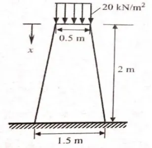
A. Structural Problem
Consider, a bridge is supported by several concrete piers, and the geometry and loads of a typical pier are shown in Fig.1. The load 20 (kN/m2) represents the weight of the bridge and an assumed distribution of traffic on the bridge.
The concrete weighs approximately 25 (kN/m3) and its
modulus is E=28*106 (kN/m2). Here, we analyze the
[image:4.612.331.560.549.668.2]displacement along the pier at different points (nodes).
Figure 1. A typical concrete pier.
Governing equation is
E
dx
du
x
dx
u
d
25
)
1
(
1
2 2
for0 ≤ x ≤ 2 (21)
With boundary conditions u(2)=0,
5
4
)
1
(
0
x
dx
du
E
x
and having a exact solution
E
x
x
x
u
3
1
ln
5
.
7
)
1
(
25
.
6
25
.
56
)
(
2
(22)
Taking the approximation function from the equation (2), it can be written as
12
,
(
)
)
(
n
i
p i i h
x
R
C
x
U
Taking number of intermittent segments (or sub domains) as 11 (i.e. n=11), order of NURBS curve as 3 (i.e. p=3). X={a=X0=0, X1, X2, …. Xn-1, Xn=b} with
non-uniform values between [a b], for a homogeneous
coordinates (weights) h1=1.12, hi=1, for i≠1 and knot
vector having 12 elements or knot values. Now the above equation can be modified as
102 3 ,
(
)
)
(
i
i i h
x
R
C
x
U
(23)Equation (23) is evaluated at xi={0, 0.0093, 0.1564,
0.2133, 0.8854, 1.5498, 1.6346, 1.7374, 1.9238, 1.9923, 2}, for i=1to 11 gives the system of (10)×(12) equations in which (12) arbitrary constants are involved. From equation (17) we get the below matrix form.
E E E
C C C C
R R
R R
R R
R R
R R
R R
R R
R R
25 . . . . 25 25
. . .
) 9923 . 1 ( )... 9923 . 1 ( ) 9923 . 1 ( ) 9923 . 1 (
. .
. .
. .
. .
. .
. .
) 1564 . 0 ( )... 1564 . 0 ( ) 1564 . 0 ( ) 1564 . 0 (
) 0093 . 0 ( )... 0093 . 0 ( ) 0093 . 0 ( ) 0093 . 0 (
) 0 ( )...
0 ( )
0 ( )
0 (
10 1 1 2
10 1
1 2
10 1
1 ,
2
10 1
1 2
10 1
1 2
(24)
[image:4.612.92.246.550.700.2]International Journal of Emerging Technology and Advanced Engineering
Website: www.ijetae.com (ISSN 2250-2459, UGC Approved List of Recommended Journal, Volume 8, Issue 4, April 2018)33
10
2 2
,
(
2
)
0
ii
i
R
C
and5
)
0
(
4
)
1
(
102 '
3
,
i
i
i
R
C
E
x
(25)
We get the system of (12) × (12) equations in which twelve arbitrary constants are involved. From equation 19, implementing the boundary conditions, equation 26 is obtained.
0 25.
. . . . 25 20
. . . . .
) 2 (
) 9923 . 1 ( )... 2 (
)... 9923 . 1 ( ) 2 (
) 9923 . 1 ( )
2 (
) 9923 . 1
( . . . .
. .
. .
. .
. .
) 1564 . 0 ( )... 1564 . 0 ( ) 1564 . 0 ( ) 1564 . 0 (
) 0093 . 0 ( )... 0093 . 0 ( ) 0093 . 0 ( ) 0093 . 0 (
) 0 (
) 0 ( )...
0 (
)... 0 ( )
0 (
) 0 ( )
0 (
) 0 (
10 1 1 2
3 , 10 10
3 , 10 1
3 , 10 1
3 , 10 2
10 1
1 2
10 1
1 2
10 3 , 10 '
1 3 , 1 '
1 3 , 1 '
2 3 , 2 '
E E
E
C C C C
R R R
R R
R R
R
R R
R R
R R
R R
R R R
R R
R R
R
(26)
It is in the form of
]
[
]
][
[
R
C
F
(27)Where [R] is matrix of basis functions, [C] is the matrix
of arbitrary constants and [F] is right side function matrix.
By solving the set of equations (27) we get the constants Ci
where i=1, 2, 3 …10. And by substituting these constant values in approximation solution equation then we get the final solution for the given problem. Now the final approximation solution is evaluated at each node
(Collocation point) i.e. xi= {0, 0.0093, 0.1564, 0.2133, …,
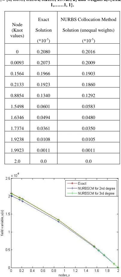
1.9923} and the values field variable u(x) at each node are calculated and provided in Table 1.
[image:5.612.340.542.156.617.2]From the Fig. 2, it is evident that the fiels variable obtaind fron NURBS collocaton method is closer to the exat solution. Further, by increasing the degree of NURBS basis from second to third degree (i.e., order from p=3 to 4) the error become negligible.
Table 1
Comparison of field variable (u) with exact solution for knot vector,
xi = {0, 0.093, 0.1564, 0.2133, 1.9923, 2} and weights hi={1.12, 1,
1,……1, 1}.
Node (Knot values)
Exact
Solution
(*10-5)
NURBS Collocation Method
Solution (unequal weights)
(*10-5)
0 0.2080 0.2016
0.0093 0.2073 0.2009
0.1564 0.1966 0.1903
0.2133 0.1923 0.1860
0.8854 0.1340 0.1292
1.5498 0.0601 0.0583
1.6346 0.0494 0.0480
1.7374 0.0361 0.0350
1.9238 0.0108 0.0105
1.9923 0.0011 0.0011
2.0 0.0 0.0
[image:5.612.49.289.271.447.2]
Figure 2. Comparison of field varible u(x) with exact and NURBS Collocation Method for second and third degree basis for unequal
International Journal of Emerging Technology and Advanced Engineering
Website: www.ijetae.com (ISSN 2250-2459, UGC Approved List of Recommended Journal, Volume 8, Issue 4, April 2018)34
B. Long cylindrical fin with insulated end
Consider a steel rod of diameter D=0.02m, length L=0.05m, and thermal conductivity k=50 (W/m-˚C) is
exposed to ambient air at T∞=20˚C with a heat transfer
coefficient β=100 (W/m2-˚C) (see Fig.3). The left end of
the rod is maintained at temperature T0=320 and other
[image:6.612.55.281.237.349.2]end is insulated. The temperature distribution along the rod at different locations (nodes) is calculated).
Figure 3: Heat transfer through a cylindrical fin with insulated end.
The governing equation is
0
2 2 2
m
dx
d
for 0 ≤ x ≤ L (28)
where,
θ
=(T-T∞), temperature gradient and.
400
4
2
kD
m
With boundary conditions
(0)=300 and0
)
05
.
0
(
dx
d
and having a exact solution
)
1
cosh(
)
20
1
cosh(
*
300
)
(
x
x
(29)Taking the approximation function from the equation (2), it can be written as
1 2 ,(
)
)
(
n i p i i hx
R
C
x
Taking number of intermittent segments (or sub domains) as 11 (i.e. n=11), order of NURBS curve as 3 (i.e. p=3). X={a=X1=0, X2, …. Xn-1, Xn=b} with non-uniform
values,Є[a b], for homogeneous coordinates (weights)
h12=0.75, hi=1 for i≠12 and knot vector having 12 elements
or knot values.
Now the above equation can be modified as
10 2 3 ,(
)
)
(
i i i hx
R
C
x
(30)Substituting the approximation function in governing equation we have
0
)
(
400
)
(
10 2 3 , 10 2 3 , ''
i i i i ii
R
x
C
R
x
C
(31)
Equation(31) is evaluated at xi ={0 0.0078 0.018 0.0213
0.0258 0.0278 0.0281 0.0347 0.0366 0.0418 0.05},for i=1,2,3,...11 gives the system of (10)×(12) equations in which twelve arbitrary constants are involved. i.e.,
0 . . . 0 0 0 . . . ) 0418 . 0 ( )... 0418 . 0 ( ) 0418 . 0 ( ) 0418 . 0 ( . . . . . . . . . . . . ) 018 . 0 ( )... 018 . 0 ( ) 018 . 0 ( ) 018 . 0 ( ) 0078 . 0 ( )... 0078 . 0 ( ) 0078 . 0 ( ) 0078 . 0 ( ) 0 ( )... 0 ( ) 0 ( ) 0 ( 10 1 1 2 10 1 1 2 10 1 1 2 10 1 1 2 10 1 1 2 C C C C R R R R R R R R R R R R R R R R (32)
Now let the approximation solution satisfy the boundary conditions. The given boundary conditions are from equation (18) and (22)
10 2 3,
(
0
)
300
i i iR
C
and0
)
05
.
0
(
10 2 3 , '
i i iR
C
(33)Rewriting the equation (32) using boundary condition equations (33), we get the system of (12) × (12) equations in which twelve arbitrary constants are involved. From equation (19) we obtain the following form.
International Journal of Emerging Technology and Advanced Engineering
Website: www.ijetae.com (ISSN 2250-2459, UGC Approved List of Recommended Journal, Volume 8, Issue 4, April 2018)35
It is in the form of
[
R
][
C
]
[
F
]
Where [R] ismatrix of basis functions, [C] is the matrix of arbitrary constants and [F] is right side function matrix. We have
1
]
][
[
]
[
C
F
R
(35)By solving the set of equations (35), we get the constants
Ci where i=1, 2, 3 …10. And by substituting these constant
values in approximation solution equation then we get the final solution for the given problem.
Now the final approximation solution is evaluated at
each node (Collocation point) i.e. xi=0, 0.0078, 0.018,
0.0213 …0.0418 and the values field variable
(x) at eachnode are calculated. The exact solution also evaluated at these points and result values of field variable
(x) are compared with each other to find out the accuracy of the NURBS collocation method.Table 2:
Comparison of field varible θ(x) with exact and nurbs collocation method with equal and unequal weights.
Node(Knot
Values) Exact Sol
NURBSCM Sol. with
Equal weights, hi=1
(B-Spline)
NURBSCM sol. with Unequal weights
0 300 300 300
0.0078 267.8705 266.9406 267.4089
0.018 235.6105 234.0371 235.1276
0.0213 227.3331 225.6986 226.9960
0.0258 217.6359 215.9371 217.5250
0.0278 213.8964 212.1777 213.8983
0.0281 213.3651 211.6435 213.3843
0.0347 203.5897 201.8194 204.0189
0.0366 201.4400 199.6677 202.0052
0.0418 197.0367 195.2576 197.9898
0.05 194.4163 192.6318 195.6852
[image:7.612.335.542.142.298.2]
Figure 4: Comparison of field varible θ( ) with exact and NURBS Collocation Method with equal and unequal weights.
From Table 2, it is clear the results obtained from NURBS Collocation Method with unequal weights is much near to exact solution compared to solution obtained using equal weights. These values are plotted in Fig. 4. So, it can be stated that the NURBS Collocation Method with unequal weights gives better approximation fit when compared to solution obtained by equal weights.
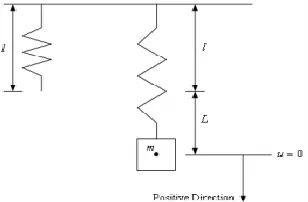
C. Damped Free Vibration of Spring
A 16 lb object stretches a spring (8/9) ft by itself. There is no damping and no external forces acting on the system.
Attached, a damper to the spring that exerts a force (Fd) of
5 lbs when the velocity is P'=2 lb/sec. (See in the Fig. 5).
Find the displacement 'u' distribution. The mass (m = 1/2)
and spring constant (s = 18). The damping coefficient (γ) is
[image:7.612.368.522.532.633.2]derived from: Fd = γ P΄ gives γ = 5/2 = 2.5.
International Journal of Emerging Technology and Advanced Engineering
Website: www.ijetae.com (ISSN 2250-2459, UGC Approved List of Recommended Journal, Volume 8, Issue 4, April 2018)36
The governing equation is 2
5
36
0
2
u
dy
du
dy
u
d
for 0 ≤ y ≤ 1 (36)
With boundary conditions u(0) = 0 and u(1) = 1 and having a exact solution
))
2
/
5
sinh(
)
2
/
5
(cosh(
*
)
2
/
119
sin(
))
2
/
(
119
sin(
*
)
(
2 / 5
e
y
y
u
y
(37)
Taking the approximation function from the equation (2), it can be written as
12
,
(
)
)
(
n i
p i i h
y
R
C
y
U
Taking number of intermittent segments (or sub domains) as 51 (i.e. n=51), order of NURBS curve as 3 (i.e.
p=3).Y={a=Y1=0, Y2, …. Yn-1, Yn=b} with non-uniform
values from [a b], for a homogeneous coordinates (weights)
hi=[1 1 1 1 1.1 1.1 1 1 1 1 1 1 1 1 1 1 1 1 0.85 0.65 0.55 1 1
1 1 1 1 1 1 1 1 1 1 1 1 1 1 1 1 1 1 0.85 0.65 0.85 1 1 1 1 1 1 1 1] and knot vector having 52 elements or knot values. Now the above equation can be modified as
502
3
,
(
)
)
(
i
i i h
y
R
C
y
U
(38)Equation (38) is evaluated at yi={0 0.0193 0.0423
0.0476 0.0839 0.0943 0.1217 0.1220 0.1378 0.1386 0.1522 0.1892 0.2312 0.2409 0.2578 0.2684 0.2815 0.3317 0.3480 0.3488 0.3531 0.3610 0.3662 0.4035 0.4494 0.4513 0.4896 0.5038 0.5864 0.5882 0.5906 0.6203 0.6246 0.6513 0.6604 0.6671 0.6751 0.7111 0.7150 0.7311 0.8068 0.8112 0.8367 0.8562 0.8770 0.8842 0.9300 0.9635 0.9730 0.9748 1.0}, for i=1 to 50 gives the system of (50)×(52) equations in which (52) arbitrary constants are involved.
Now let the approximation solution satisfy the boundary conditions. The given boundary conditions are from equation (18)
502 3 ,
(
0
)
0
i i i
R
C
and(
1
)
1
50
2 3 ,
i i
i
R
C
(39)Rewriting the equation (38) using boundary condition equations (39), we get the system of (52) × (52) equations in which (52) arbitrary constants are involved. From equation (19),
1 0 . . . 0 0 0 0
. . . . .
) 1 (
) 9748 . 0 (
)... 1 (
)... 9748 . 0 (
) 1 (
) 9748 . 0 (
) 1 (
) 9748 . 0
( . . . .
. .
. .
. .
. .
) 0423 . 0 ( )... 0423 . 0 ( ) 0423 . 0 ( ) 0423 . 0 (
) 0193 . 0 ( )... 0193 . 0 ( ) 0193 . 0 ( ) 0193 . 0 (
) 0 (
) 0 (
)... 0 (
)... 0 (
) 0 (
) 0 (
) 0 (
) 0 (
50 1
1 2
3 , 50 50 3
, 1 1 3
, 1 1 3
, 2 2
50 1
1 2
50 1
1 2
50 3 , 50 1
3 , 1 1
3 , 1 2
3 , 2
C C C C
R R
R R
R R
R R
R R
R R
R R
R R
R R
R R
R R
R R
(40)
It is in the form of
[
R
][
C
]
[
F
]
(41)
Where [R] is matrix of basis functions, [C] is the matrix
of arbitrary constants and [F] is right side function matrix.
By solving the set of equations (41) we get the constants Ci
where i=1, 2, 3 …50. And by substituting these constant values in approximation solution equation then we get the final solution for the given problem.
Now, the final approximate solution is evaluated at each
node (Collocation point) i.e., yi={0, 0.0193, 0.0423,
0.0446, 0.0839, 0.0943 …0.9748} and the values field variable u(y) at each node are calculated.
[image:8.612.342.537.501.656.2]From Fig.6, it can be stated that the NURBS Collocation method with unequal weights gives better approximation fit when compared to solution obtained by equal weights.
International Journal of Emerging Technology and Advanced Engineering
Website: www.ijetae.com (ISSN 2250-2459, UGC Approved List of Recommended Journal, Volume 8, Issue 4, April 2018)37
V. CONCLUSIONS
In this work, an attempt has been made to use the NURBS basis functions as the basis functions in the collocation method. A non-uniform knot vector was used to obtain the first, second and third degree NURBS basis functions. The derivatives of basis functions were obtained from recursive formula. The method has been applied for solving 1-D problems. The results were compared with exact solution and found that the present method is in good agreement with exact solution. It can be concluded that NURBS basis functions give good results compared to B-Spline basis functions.
REFERENCES
[1] Reddy J.N ―An Introduction to the Finite Element Method‖, 3rd ed., Tata McGraw-Hill Edition, New Delhi, 2005.
[2] Sridhar Reddy, CH, Rajashekhar Reddy Y and Srikanth, P ―Application of B-spline Finite Element Method for One Dimensional Problems‖, International Journal of Current Engineering and Technology, April-2014.
[3] Hughes, T.J.R., Cottrell, J.A. and Bazilevs, Y. ‗‗Isogeometric analysis: CAD, finite elements, NURBS, exact geometry and mesh refinement‘‘, Comput. Methods Appl. Mech. Engg., 194(39–41), pp. 4135–4195 2005.
[4] Sharanjeet Dhawan and Sheo Kumar, "A Galerkin B-Spline Approach to One Dimensional Heat Equation", International Journal of Research and Reviews in Applied Sciences, Volume 1, Issue 1, 2009.
[5] Samuel Jator and Zachariah Sinkala. ―A high order B-spline collocation method for linear boundary value problems‖ Eslevier, Applied Mathematics and Computation 191, 2007,100–116. [6] Botlla, O, ―On a collocation B-spline method for the solution of the
Navier–Stokes equations‖, Pergamon, Computers & Fluids 31 2002, p. 397–420.
[7] Bharti Gupta and V.K. Kukreja, ―Numerical approach for solving diffusion problems using cubic B-spline collocation method‖ Eslevier, Applied Mathematics and Computation Vol. 219, 2012, p. 2087–2099.
[8] Kasi Viswanadham . K.N.S. and Showri Raju. Y, "Quartic B-Spline Collocation Method for Fifth Order Boundary Value Problems", International Journal of Computer Applications (0975– 8887) Volume 43– No.13, April 2012.
[9] Dabral. V, Kapoor. S and Dhawan. S, " Numerical Simulation of one dimensional Heat Equation: B-Spline Finite Element Method", Indian Journal of Computer Science and Engineering (IJCSE). Vol.2 No.2, 2011.
[10] Suresh. A, Yella Reddy. CH, NURBS based Finite Element Approach for One Dimensional Problems, Intrnational Journalof Engineering Research & Technology, 5(08), 2016, 494-499. [11] David F. Rogers and J. Alan Adams, ―Mathematical Elements for