STATISTICAL MODELLING OF TRAINING AND
PERFORMANCE USING POWER OUTPUT AND
HEART RATE DATA COLLECTED IN THE FIELD
PhD Thesis
Naif Mohammed Alotaibi
University of Salford, Manchester, UK
Submitted in Partial Fulfilment of the Requirements of
the Degree of Doctor of Philosophy
II
List of Contents
List of Contents ... II List of Figures ... VI List of Tables ... VIII Acknowledgement ... XI Abstract ... XII
CHAPTER ONE
... 11
INTRODUCTION
... 11.1 Background ... 1
1.2 Research Motivation... 3
1.3 Aim and Objectives ... 3
1.4 Research Contributions ... 4
1.5 Research Question ... 4
1.6 Thesis Structure ... 4
CHAPTER TWO
... 52
DATA DESCRIPTION
... 52.1 Introduction ... 5
2.2 Training Data ... 5
2.3 Power Meters ... 6
2.4 Heart Rate Monitoring... 7
2.5 Power Output Monitoring ... 11
2.6 Summary ... 14
CHAPTER THREE
... 153
MEASURING PERFORMANCE AND TRAINING
... 153.1 Introduction ... 15
III
3.3 Measuring Training Load ... 17
3.3.1 Training Impulse (TRIMP) ... 17
3.3.2 Training Stress Score (TSS) ... 20
3.4 Banister Model ... 23
3.5 Over-Training ... 24
3.6 Measuring Performance ... 25
3.6.1 Introduction... 25
3.6.2 A Performance Measure based on the Relationship between Power output and Heart Rate ... 27
3.6.3 A Modified Performance Measure based on the Relationship between Power output and Heart Rate ... 31
3.7 Summary ... 31
CHAPTER FOUR
... 364
RELATING TRAINING TO PERFORMANCE
... 364.1 Introduction ... 36
4.2 The Parameters of the Performance – Training Model ... 36
4.3 Statistical Discussion of the Training Effect ... 39
4.4 Practical Discussion of the Training Effect ... 39
4.5 Discussion of Results ... 41
4.6 Summary ... 43
CHAPTER FIVE
... 525
A MODIFIED TRAINING - PERFORMANCE MODEL
... 525.1 Introduction ... 52
5.2 Relating Training to Performance ... 52
5.3 Statistical Discussion of the Training Effect ... 53
5.4 Practical Discussion of the Training Effect ... 54
5.5 Discussion of Results ... 55
IV
CHAPTER SIX
... 616
OTHER PERFORMANCE MEASURES
... 616.1 Introduction ... 61
6.2 Performance Measure using the 75th Percentile of the Power Output... 61
6.3 Relating Training to the Performance Measure ... 66
6.3.1 Statistical Discussion of the Training Effect ... 66
6.3.2 Practical Discussion of the Training Effect ... 67
6.3.3 Discussion of Results ... 67
6.4 Performance Measure using Maximum Power ... 71
6.5 Relating Training to the Performance Measure ... 75
6.5.1 Statistical Discussion of the Training Effect ... 75
6.5.2 Practical Discussion of the Training Effect ... 76
6.5.3 Discussion of Results ... 76
6.6 Critical Power Concept ... 80
6.6.1 Discussion of Results ... 83
6.7 Relating Training to the Performance Measure ... 96
6.7.1 Statistical Discussion of the Training Effect ... 96
6.7.2 Practical Discussion of the Training Effect ... 96
6.7.3 Discussion of Results ... 97
6.8 Summary ... 98
CHAPTER SEVEN
... 1017
COMPARISON OF PERFORMANCE MEASURES
... 1017.1 Introduction ... 101
V
CHAPTER EIGHT
... 1078
DISCUSSION AND CONCLUSIONS
... 1078.1 Introduction ... 107
8.2 Conclusions ... 108
8.3 Limitations of our Study... 111
8.4 Future Work ... 112
Appendix 1: Correlation of power output and heart rate at different lags ... 115
Appendix 2: Power output versus heart rate for all training sessions ... 125
Appendix 3: Heart rate versus power output for all training sessions ... 132
Appendix 4: The estimated parameters of the model between power output and heart rate ... 139
Appendix 5: The estimated parameters of the model between heart rate and power output for each rider ... 145
Appendix 6: Estimate of varied from session to session ... 153
Appendix 7: Estimate of varied from session to session for critical power Model (2) 157 Appendix 8: Estimate of varied from session to session for critical power Model (1) 161 Appendix 9: Estimates of and standard error of both parameters for all sessions ... 165
Appendix 10: Fitted line of for the relationship between power output and duration ... 182
VI
List of Figures
Figure 2-1 An example of SRM monitor and SRM power meter ... 7
Figure 2-2 Examples of heart rate (bpm) from two training sessions for rider (1) ... 7
Figure 2-3 The duration of each training session for each rider ... 8
Figure 2-4 The average heart rate for each training session for each rider, with maximum and minimum average heart rate ... 9
Figure 2-5 The histogram of the entire heart rate measurements for each rider ... 10
Figure 2-6 Factors influencing cycling power output and consequential velocity ... 11
Figure 2-7 Examples of power output (watts) from two training sessions for rider 1 ... 11
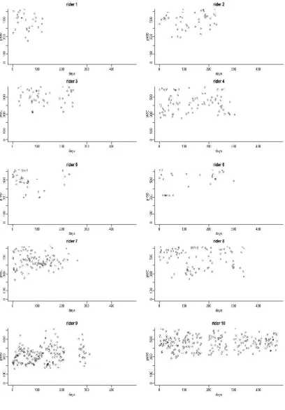
Figure 2-8 The average power output for each training session for each rider, with maximum and minimum average power output ... 12
Figure 2-9 The histogram of the entire power output measurements for each rider ... 13
Figure 3-1 The modified training impulse (TRIMP), equation (3.2) for each rider for each session ... 19
Figure 3-2 Training stress score (TSS) for each session for each rider ... 21
Figure 3-3 Training stress score (TSS) against modified training impulse (TRIMP) for each rider ... 22
Figure 3-4 ATE given one unit of training load on day 1 with parameters =30, =7, =1.5 and =1 ... 23
Figure 3-5 ATE given one unit of training load once per week for 25 weeks with parameters =30, =7, =1.5 and =1 ... 23
Figure 3-6 Power output and heart rate vs time for rider 3 in session 13, from minute 0 to minute 100 ... 26
Figure 3-7 Power output and heart rate vs time for rider 3 in session 13, from minute 40 to minute 65 ... 26
Figure 3-8 Power output and heart rate vs time for rider 3 in session 13, from minute 30 to minute 40 ... 26
Figure 3-9 Power output vs heart rate with fitted line for rider 3 in a single session ... 28
Figure 3-10 Performance measure for each session for each rider ... 29
VII
Figure 3-12 Heart rate vs power output with fitted line for rider 1 in a single session ... 32
Figure 3-13 Performance measure for each session for each rider ... 33
Figure 3-14 Performance measure for each session for each rider ... 34
Figure 3-15 Performance measure for each session for each rider ... 35
Figure 4-1 Two plots for each rider: left (symbols) vs time in days and ATE (line) when =2 vs time in days; right vs ATE (all sessions) ... 44
Figure 4-2 Two plots for each rider: left (symbols) vs time in days and ATE (line) when = 2 vs time in days; right vs ATE (all sessions) ... 46
Figure 4-3 Two plots for each rider: left (symbols) vs time in days and ATE (line) when 2 vs time in days; right vs ATE (all sessions) ... 48
Figure 4-4 Two plots for each rider: left (symbols) vs time in days and ATE (line) when 2 vs time in days; right vs ATE (all sessions) ... 50
Figure 5-1 Two plots for each rider: left (symbols) vs time in days and ATE (line) vs time in days; right vs ATE (all sessions) ... 57
Figure 5-2 Two plots for each rider: left , (symbols) vs time in days and ATE (line) vs time in days; right , vs ATE (all sessions) ... 59
Figure 6-1 (in watts) varied from session to session for each rider ... 62
Figure 6-2 The confidence interval of the (in watts) for all sessions for each rider .... 64
Figure 6-3 Two plots for each rider: left , (symbols) vs time in days and ATE (line) vs time in days; right , vs ATE (all sessions) ... 69
Figure 6-4 Observed power output against duration (points) and fitted power output and duration curve for a single session for rider 1 ... 71
Figure 6-5 Two plots for each rider: left , (symbols) vs time in days and ATE (line) vs time in days; right , vs ATE (all sessions)... 78
Figure 6-6 An example of the power output and duration with CP ... 81
Figure 6-7 Observed power output and duration, and fitted critical power curve for Model 1 for each rider for all sessions ... 84
Figure 6-8 Observed power output and duration, and fitted critical power curve for Model 2 for each rider for all sessions ... 86
VIII
Figure 6-10 The confidence intervals of the parameter for each session for critical power Model 1 ... 90 Figure 6-11 Estimate of for each session for each rider for critical power Model 2 ... 92 Figure 6-12 The confidence intervals of parameter for each session for crtical power Model 2 ... 94 Figure 6-13 Two plots for each rider: left , (symbols) vs time in days and ATE (line) vs time in days; right , vs ATE (all sessions) ... 99
List of Tables
Table 2-1 Summary data for each rider ... 5 Table 2-2 Maximum heart rate and resting heart rate for each rider ... 8 Table 3-1 The correlation coefficient between training stress score (TSS) and modified training impulse (TRIMP) for each rider ... 20 Table 3-2 Various percentiles of power output data for each rider ... 28 Table 3-3 Various percentiles of heart rate data for each rider ... 32 Table 4-1 Estimated parameters with standard errors of the model for performance measure
and =2 for each rider, with the t statistic and p value for the test of β=0. ... 38 Table 4-2 Estimated parameters with standard errors of the model for performance measure
and =2 for each rider, with the t statistic and p value for the test of β=0. ... 38 Table 4-3 Estimated parameters with standard errors of the model for performance measure
when for each rider, with the t statistic and p value for the test of β=0. ... 38 Table 4-4 Estimated parameters with standard errors of the model for performance measure
when for each rider, with the t statistic and p value for the test of β=0. ... 39 Table 4-5 The coefficients of the model between power output and heart rate from the last 60 days ... 40 Table 4-6 Performance gain and the ATE change for each rider at performance measure
and =2 ... 40 Table 4-7 PPerformance gain and the ATE change for each rider at performance measure
and =2 ... 40 Table 4-8 Performance gain and the ATE change for each rider at performance measure
IX
X
XI
Acknowledgement
XII
Abstract
This thesis develops statistical models of performance and training that make use of power output and heart rate data. These data were collected during training and competition, and were recorded every five seconds using a power meter and heart rate monitor. Using these data, we estimate the parameters of the Banister model of training and performance. In principle, knowledge of these parameters allows one to provide quantitative decision support for the scheduling of training in advance of a major competition.
The methodology proceeds in a number of steps. In the first, measures of both training and performance must be specified. The training experienced by an athlete in a single session, the training load, can be measured in a number of ways. We use the TRIMP measure. This measure in its simplest form is essentially the total number of heart beats in a training session. Then the training loads of successive sessions are accumulated into a single measure of training up to time t. This we term the accumulated training effect (at time t). Performance during a session at time t is defined as a function of the power output observed during the session. We consider various performance measures and describe these in detail in the thesis. Then in the second step, we relate the performance at time t to the training load up to time t using a regression model, estimating the parameters of the performance training relationship. The final step is the training optimisation step, whereby the known training-performance model parameters can be used to specify training loads up to time T that will maximise (in expectation) the performance at time T.
We demonstrate the methodology using the training data histories of ten competitive male cyclists. As each athlete has his own specific characteristics, we should focus on optimising training and performance individually. We compare and contrast the different performance measures that we propose.
1
1
INTRODUCTION
1.1
Background
The fundamental aim of this thesis is to develop a model that relates performance to training in cycling. The purpose of this model is to allow training to be quantified and planned systematically in order to improve the capability of an athlete in advance of a particular competition.
Training in sport, in particular, is the approach through which an athlete can improve his or her individual performance. It builds specific abilities and attributes that would optimise his or her overall performance required in specific competitions (Fister et al., 2015). The process of training essentially involves carrying out the same exercises numerous times to develop the skills, strength and endurance of the athlete, which lead to increased physical performance. Cycling training mainly aims to increase the ability of a rider to produce a power output or speed over a specified time or distance. By monitoring training sessions and performances during races with the help of a power meter and heart rate monitor, one can attempt to understand and model the relationship between training and performance (Passfield et al., 2016). Banister et al. (1975) suggested that a systematic theory can be adopted to model the response of an athlete to training. This paper suggested that there are two opposing responses to a training load: the positive fitness response and the negative fatigue response. This idea was reinforced later by Calvert et al. (1976), Morton (1997), and Busso (2003) who expressed the process of training as an impulse oriented mathematical model. The basic characteristic of their model was the mathematical link between preparedness and the training impulse (Busso & Thomas, 2006).
Hellard et al. (2006a) observed that useful information can be obtained from a modelling oriented approach and that this will be helpful in shaping individual training programs. However, Taha and Thomas (2003) observed that models so far developed did not relate to strictly physiological mechanisms. These models are also not able to differentiate between the particular impacts of various impulses of training. Moreover, inter-subject and inter-study variance limit the potential for developing and applying a general model, so that Jobson et al. (2009) observed that the prediction of performance output using training input was still an unsolved issue. Having regard to this, we evaluate whether the individual parameter values of the performance-training relationship can be deduced from the link between heart rate and power output data.
2
under/over training, aiming to strike the optimum balance. However, for the model to be specific rather than just indicative, both performance and training must be quantified, and the parameters of the Banister model must be estimated. A number of studies have estimated Banister model parameters in different types of sports (Busso et al., 2002; Calvert et al., 1976; Hayes & Quinn, 2009; Wood et al., 2005), but these studies do not report the precision of estimates of parameters.
In the PhD study of Shrahili (2014), a quantitative model was established to relate training to performance based on the Banister model (Banister et al., 1975). We extend that work to consider other alternative performance measures and to consider the effect of cardiovascular drift on performance measurement (Wingo et al., 2005). Cardiovascular drift is the gradual increase in heart rate during exercise at a fixed workload (Hamilton et al., 1991; Morales-Palomo et al., 2017). The performance measures are compared in terms of their statistical and practical significance. The selection of a performance measure is then down to athlete choice, albeit with the support of the analysis that this thesis provides. We also consider the usefulness of the Banister model for optimising training in advance of a particular competition.
Thus in our study, we also use the Banister model to specify the accumulated training effect at a time . The model has a number of parameters that must be estimated for an individual rider. These parameters are necessary for using the model to plan training for each rider. We use power output and heart rate data collected in the field to make this estimation possible.
Our method includes some stages that must be achieved. Firstly we require two measures, those of training and performance. The training measure that we consider is associated with the training impulse TRIMP measure. In its most basic form, this measure is the sum of the total heart beats of the athlete during the session. The training loads of consecutive sessions are combined to determine a measurement of training up to time t.
This is termed the accumulated training effect at time t. The performance in a session at time t is determined as a function of the power output achieved throughout the session. Various performance measures are considered and explained in detail in the thesis. Importantly, we suppose performance is measured with error. We quantify this error in a statistical model. In this way, we distinguish between the notion of preparedness of Busso and Thomas (2006), which is the expectation of performance, and performance itself which is a random variable with this expectation. Secondly, the performance calculated at time t
is related to the training load up to time t with the use of a regression model. In this method, the parameters of the relationship between performance and training are estimated. Lastly, the parameters estimated are utilised to specify the training loads required preceding time t to maximisetheathlete‟sperformanceattimeT.
3
technical factors (Wakayoshi et al., 1995), speciality (Stewart & Hopkins, 2000) and psychological factors (Saw et al., 2015).
Finally, here, we make a brief statement of the methodology in this thesis. Primarily this PhD is concerned with the field of statistics, and in particular, we use statistical modelling to quantify the uncertainty in estimates of parameters that arises because of the limited information that data provide about the real, underlying relationships. This point about uncertainty in the training-performance relationship has been not considered by the sports science literature to date. A statistical model is a set of assumptions about the generation of observed data and, in principle, we test the veracity of these assumptions given the data available. Statistical modelling then proceeds by accepting the model or modifying it according to the evidence for the model, and finally using the model to make deductive statements. In our case, these deductive statements concern the nature of the training-performance relationship.
1.2
Research Motivation
The quantification of the relationship between training and performance is an unsolved problem. This is the motivation of this study. In particular, if a coach and an athlete know that one additional unit of training on day t prior to competition on day T produces β units of improvement in performance on day T, this would provide very useful information for planning training. This is based on the presumption that better performance is desirable because better performance implies a higher chance of winning. This is the axiom of training.
Cycling lends itself to the statistical methodology we develop because power output is directly measurable and power output data can be and is routinely collected by riders using power meters and cycle computers. In other sports, the measurement of power output (and data collection) is more difficult.
1.3
Aim and Objectives
The aim of this study is to develop a model that can be used to optimise a training programme for an individual cyclist. To do so, we use power output and heart rate data collected every five seconds in training and competition. To achieve this aim, we have the following objectives:
To develop statistical models that link power output to heart rate. Through these models, a performance measure can be specified and calculated for each session for each rider.
To develop a statistical model that relates performance to training.
To apply these models to the power output and heart rate data of a number of athletes. To compare different performance measures in terms of their statistical and practical
significance.
4
1.4
Research Contributions
The main contributions of this thesisareasfollows:
To introduce various measures of performance, calculated using power output and heart rate data, where these data are recorded using a power meter and heart-rate monitor, and where each one of these performance measures depends on a specific performance concept.
To relate these performance measures to a training measure, which is defined using the Banister model, and through this relationship, to estimate the Banister model parameters for each performance measure.
To compare the different performance measures in terms of the statistical and practical significance of the models pertaining to them, in order to suggest a best measure of performance that a cyclist should use to optimise performance at a future competition. To demonstrate more realistically that while different performance measures can be
specified, a methodology used to estimate the Banister model parameters that are appropriate for them is common to the various different performance measures.
To present the idea that performance is a random variable and therefore that the performances of an athlete in a session (training or competition) is different from the readiness to perform (preparedness) of the athlete at the time of this session.
1.5
Research Question
We formulate the research question as:
Can a practical method be established that quantitatively relates performance to training in cycling using power output and heart rate data collected in the field?
1.6
Thesis Structure
5
2
DATA DESCRIPTION
2.1
Introduction
In this chapter, we describe the data that we use in this thesis. These data are power output and heart rate collected every five seconds during training and competitions. A summary for each athlete is presented. Moreover, how data such as these are collected is described, and the instrument (SRM power meter) that is used by riders to collect data is illustrated. Furthermore, some examples of heart rate and power output from two training sessions for one rider are presented to show the format of the data.
2.2
Training Data
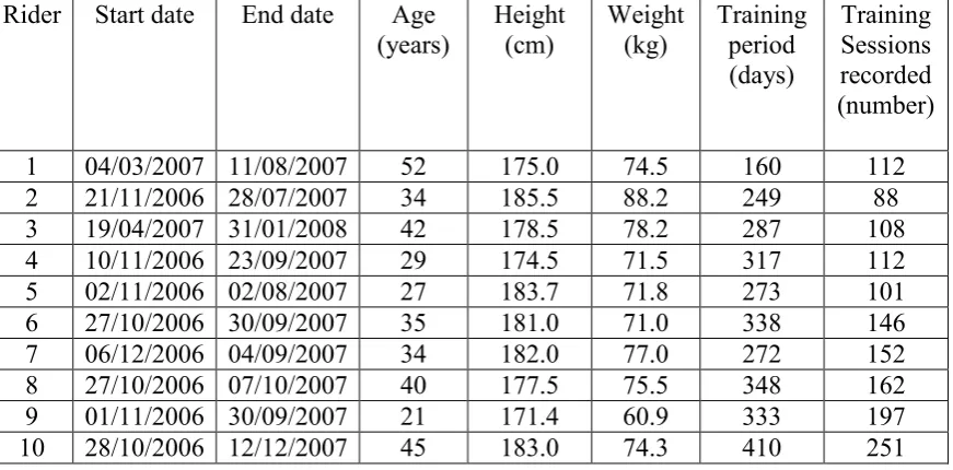
[image:17.595.90.526.523.738.2]Our methodology is illustrated using data from ten competitive, male road cyclists. These riders collected data on power-output and heart rate for nominally all their sessions (training, testing and competition) over a period in 2006-2008. Missing data on a particular day might be due to either a lack of recording or no ride that day. At the time the data were collected the ages, masses, and heights of the riders were as in Table 2.1. Measurements of power output were recorded every 5 seconds using power-meter cranks (SRM, Julich, Germany). The riders gave written, informed consent for their data to be used in this study, and the data collection received ethics-committee approval at the University of Kent and was carried out according to the principles of the Declaration of Helsinki (World Medical Association, 2013).
Table 2-1 Summary data for each rider Rider Start date End date Age
(years) Height (cm) Weight (kg) Training period (days) Training Sessions recorded (number)
1 04/03/2007 11/08/2007 52 175.0 74.5 160 112
2 21/11/2006 28/07/2007 34 185.5 88.2 249 88
3 19/04/2007 31/01/2008 42 178.5 78.2 287 108
4 10/11/2006 23/09/2007 29 174.5 71.5 317 112
5 02/11/2006 02/08/2007 27 183.7 71.8 273 101
6 27/10/2006 30/09/2007 35 181.0 71.0 338 146
7 06/12/2006 04/09/2007 34 182.0 77.0 272 152
8 27/10/2006 07/10/2007 40 177.5 75.5 348 162
9 01/11/2006 30/09/2007 21 171.4 60.9 333 197
6
The data were not collected specifically for the study in this thesis. The data were collected by sports scientists at the University of Kent as part of an extended study of training and performance that received EPSRC support through grant number EP/F006136/1. Collaboration on this grant led to the opportunity to use these data for the study in this thesis. We are satisfied that the data are robust.
The data then are secondary data. A consequence of this is that, for our study, it would not have been possible to extend the data with contextual information, relating to, for example, qualitative reporting of: the nature of sessions; descriptions of any activity between sessions; periods of illness and injury if applicable; etc. To collect data specifically for this thesis would have been very difficult, and beyond its scope. This difficulty arises principally because athletes (and coaches) are protective of data about their performance. The riders whose data were used in this study were developing riders and had the trust of the scientists at the University of Kent. The riders are anonymised throughout this thesis.
2.3
Power Meters
7
Figure 2-1 An example of SRM monitor and SRM power meter
2.4
Heart Rate Monitoring
Heart rate monitors (HRMs) have been used as popular training tools among coaches and athletes for a long time. Their cost-effectiveness and easy application have made HRMs a very common tool in measuring the extent of exercise and training load (Achten & Jeukendrup, 2003; Jeukendrup & Diemen, 1998; Mazzoleni et al., 2016). Furthermore, HRMs are also useful to identify overtraining (Achten & Jeukendrup, 2003). The use of HRMs for estimating exercise intensity, energy exhaustion, and exercise load in cycling competitions has been researched for many years (Andez-Garcia et al., 2000; Impellizzeri et al., 2005; Mujika & Padilla, 2001). At the same time, the use of HRMs has some barriers. Within and between sessions, variations in the heart rate occur due to multiple factors such as hydration status, ambient temperature, cardiovascular drift (Rowell et al., 1996), and altitude (Achten & Jeukendrup, 2003). Understanding these factors is essential for analysing appropriately the heart rate data accumulated throughout training.
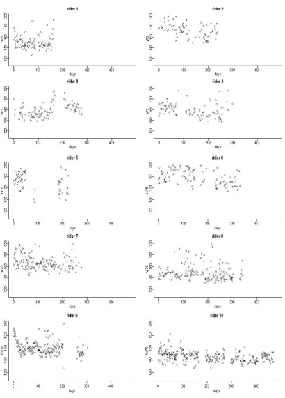
Heart rate is typically measured using a chest strap monitor that interfaces with a recording device. In our data, heart rate was recorded every 5 seconds. Examples of heart rate recorded every 5 seconds from two training sessions for rider (1) are shown in Figure 2.2. Maximum heart rate and resting heart rate for each rider in our study are shown in Table 2-2. The duration of each training session for each rider is shown in Figure 2.3. Furthermore, the average heart rate for each training session with maximum and minimum average heart rate are for each rider shown in Figure 2.4. Figure 2.5 presents the histogram of the entire heart rate measurements for each rider.
8
Table 2-2 Maximum heart rate and resting heart rate for each rider Rider Rider
1 180 45 6 187 39
2 203 48 7 187 49
3 182 45 8 173 42
4 192 42 9 192 53
5 184 42 10 176 42
9
10
11
2.5
Power Output Monitoring
Power output has been considered as the most direct measure for describing performance in cycling (Stannard et al., 2015; Vogt et al., 2006).This is because it gives a measurement or feedback instantly. Many sport scientists and coaches now use power output instead of heart rate to specify training intensity in cycling (Duc et al., 2007). Power output can be estimated by using mathematical models, or measured directly on the cyclist‟s bicycle using mobile power meters (Martin et al., 1998; Olds, 2001). We described the SRM power meter in section 2.3. Generating and sustaining the power output is considered a vital factor for athletes (Soriano et al., 2015).Various factors contribute to power output such as nutrition fitness, bike design, and riding position. Other factors can be seen in Figure 2.6 (Atkinson et al., 2007).
Figure 2-6 Factors influencing cycling power output and consequential velocity
(Atkinson et al., 2007)
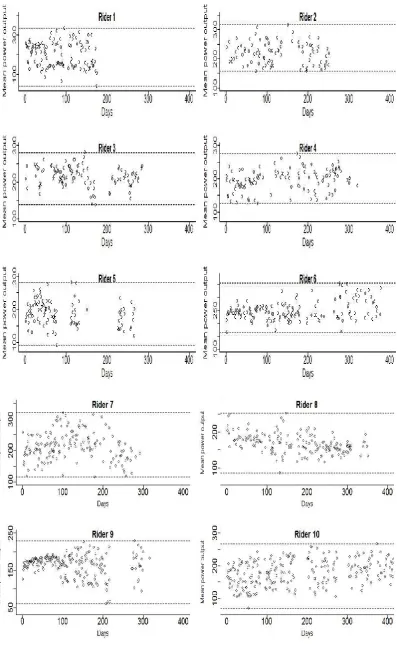
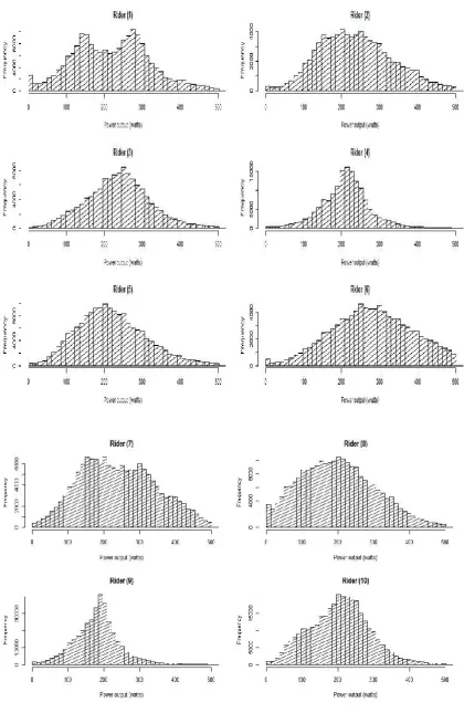
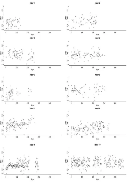
In our data, power output was measured using SRM cranks. Examples of power output recorded every five seconds from two training sessions for rider (1) are shown in Figure 2.7. The average power output for each training session for each rider with maximum and minimum average is shown in Figure 2.8. Figure 2.9 presents the histogram of the entire power output measurements for each rider.
12
13
14
2.6
Summary
15
3
MEASURING PERFORMANCE AND TRAINING
3.1
Introduction
In this chapter, we describe measures of training and performance in general and in particular. We review the literature on training and performance measures. We describe the particular measures that we use initially in our study. For training, this is the accumulated training effect at time t, which is denoted (ATE). This quantity quantifies the training load accumulation over time. For performance measurement, we describe a measure that is a function of power output and heart rate. These latter quantities are measured in the field, that is, in training and competition using a power meter and a heart rate monitor. These measures will be used in chapter 4 to estimate the relationship between training and performance.
3.2
The Relationship between Training and Performance
Knowledge of the relationship between training and performance is important to athletes and coaches for determining the optimum amount and period of training. This knowledge can enhance the performance of the athlete (Avalos et al., 2003; Foster et al., 1996; Gabbett et al., 2014). In a fundamental contribution, a mathematical model was proposed by Banister et al. (1975) that aims to describe the response of the athlete to particular training stimuli. The model proposes that readiness to perform or preparedness is the result of a positive response component (fitness) and a negative response component (fatigue). Nonetheless, these studies are qualitative rather than quantitative.
Studies have investigated the relationship between training and performance as analogous to the dose–response relationship (Morton, 1997). Moreover, some studies indicate that the primary aim of investigating such a relationship is the prescription of training stimuli that enhances the potential of an athlete to perform better by maximising the positive effects of training such as fitness, improvement in body composition, burning fat and increasing muscle mass and minimising the negative effects of training such as fatigue, stress, and injury (Borresen & Lambert, 2009; Morton, 1997).
16
(Mujika et al., 1995; Scrimgeour et al., 1986). However, that a positive relationship is reported is not surprising.
Foster et al. (1996) studied the relationship between training and performance among 56 cyclists, runners and speed skaters during 12 weeks of training. They observed that a ten-fold increase in load of training resulted in a nearly 10% increase in performance. Again, the precision of this finding is not given. However, it has also been noted that increasing the dosage of training can also sometimes lead to negative effects on performance. Additionally, it can also result in injury, fatigue, stress, and illness when the dosage of training is at its highest level (Foster, 1998; Gabbett, 2004). Qualitative approaches have been used by many researchers in order to find a relation between training and performance (Grazzi, et al. 1999; Stewart & Hopkins, 2000).
However, Banister and his colleagues were the first to attempt to model the relationship between training and performance. Banister et al. (1975) suggested a model which the benefit and detriment of training is described. Moreover, a system model with the ability to relate athletic performance profiles to training profiles was proposed by these authors. This model will be explained in more detail. We aim to utilise the Banister model to find the relationship between performance and training over time with the use of data accumulated over an extended period of training. To use the Banister model, a measure of training load and performance must be known. To optimiseathletes‟training, and in doing so maximising their future performance, the parameters of Banister model have to be available. Few studies have been able to relate training to performance quantitatively. Even though this is the case, there are a few such studies that were conducted prior to the present study.
For example, Hellard et al. (2006) conducted a study for swimming. Nine leading swimmers, of whom 5 were females and 4 were males, took part in the research, which was carried out over a one year period. Actual performances during competitions were measured during the study period. The parameters of the Banister model were estimated for every swimmer with the use of the nonlinear least squares method among actual and modelled performances. The values of the parameters were reported as =38 days and =19 days. The Banister model was applied to different sports by Morton et al. (1990), particularly for running. The values of the parameters and were reported as 45 and 15 days respectively. Precision of estimates was not reported.
Busso et al. (1997) reported the Banister model parameter estimates for cycling. Two subjects took part in a 16-week study. To determine the model parameters, they utilised the least squares method between actual and modelled performances. The values of the parameter were reported as60 days for both of the cyclists, and the values of the parameter were reported as 4 days for subject one and 6 days for subject two. Again, the precision of estimates was not reported.
17
have been explained focus primarily on the processes of the model without having regard to the standard of the input data.
Thus, in this thesis, one of our purposes is to estimate the parameter values of the Banister model for cycling, and to provide the precision of the estimates. Unlike previous studies, using a different approach, we develop new models to estimate these parameters using power output and heart rate data collected in the field. This will be explained in chapter 4.
3.3
Measuring Training Load
A number of methods have been utilised to quantify training load, such as diaries and questionnaires (Lambert et al., 2002; Shephard, 2003), direct observation (Foster et al., 2001; Hopkins, 1991) and physiological monitoring in terms of heart rate (Achten & Jeukendrup, 2003; Robinson et al., 1991). It has also been proposed to use indices of training stress, such as training impulse that uses heart rate measurements and training load (Morton et al., 1990). Despite the fact that physiological adaptation is documented adequately with respect to training in the literature, its influence on performance is not yet accurate (Borresen & Lambert, 2009; Jobson et al., 2009). Despite these developments, focus on training impulse (TRIMP) as the most suitable measure of training remains. Therefore, we use TRIMP to quantify training load. In the next section, this measure is discussed in more detail.
3.3.1 Training Impulse (TRIMP)
The training impulse (TRIMP) measure has been established to evaluate the volume or amount of training undertaken in any one given bout (Morton, 1997). Banister et al (1975) and Banister and Calvert (1980) presented the training impulse measure (TRIMP) as follows
̅̅̅ (3.1) where D is the duration of the training session in minutes and ̅ is the average heart rate during the session in beats per minute. Thus this simple measure is the total number of heart beatsinasession.Itcanbeinterpretedasanathlete‟s heart rate response to training over the duration of the training session (Borresen & Lambert, 2009). This equation was further modified by Morton et al. (1990) to
(3.2) where is as above (duration), is thefraction of heart rate reserve, and Y is the factor
that gives higher weight to high heart rates during a session. The heart rate reserve is given by
( ) ( ),
where is the average heart rate in a training session during exercise. and
18
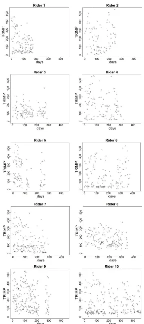
A number of studies have proposed values for the TRIMP parameters (Akubat & Abt, 2011; Morton et al., 1990; Stagno et al., 2007). The values of a and b were reported as 0.1225 and 3.9434 respectively in the study of Stagno et al. (2007). They estimated these values by fitting an exponential line for the blood lactate concentration against the fractional elevation in heart rate for eight participants. In our study, we use the modified TRIMP, equation (3.2), with the values and reported by Borresen and Lambert (2009). We use these values in order to maintain continuity with the work of Shrahili (2014). The modified training impulse (TRIMP) for each session for each rider is shown in Figure 3.1.
19
20
3.3.2 Training Stress Score (TSS)
Thetrainingstressscore(TSS)systemwasmodelledonBanister‟smodelfortraining impulse. It relies on the concept of Normalized Power (NP). TSS was used to quantify the training load in running (McGregor et al., 2009) and cycling (MacLeod & Sunderland, 2009). This measure is defined as follows:
( )/( ) (3.3)
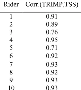
[image:32.595.233.376.400.559.2]where is the duration of the activity in seconds and is calculated for a session. The functional threshold power ( ) is defined as the maximal power that can be continued by the individual for one hour. This number is individual for each athlete. The training stress score (TSS) for each rider for each session in our study is shown in Figure 3.2. The training stress scores (TSS) and training impulses (TRIMP) for each session for each rider are shown in Figure 3.3. The correlation coefficient between training stress score (TSS) and training impulse (TRIMP) for each rider is presented in Table 3-1. Table 3-1 and Figure 3.3 show very strong positive correlation between TRIMP and TSS.
Table 3-1 The correlation coefficient between training stress score (TSS) and modified training impulse (TRIMP) for each rider
Rider Corr.(TRIMP,TSS)
1 0.91
2 0.89
3 0.76
4 0.95
5 0.71
6 0.92
7 0.93
8 0.92
9 0.93
21
22
23
3.4
Banister Model
Banister et al. (1975) proposed a model for the accumulation of training. This model specifies the training effect at time . The Banister model was simplified by Calvert et al. (1976) to include two components, which are fitness (positive impact) and fatigue (negative impact). These components include parameters that must be estimated for an individual athlete in order to optimise training.
The Banister model is proposed to measure the accumulated training effect over a number of sessions as:
∑ ( ) ⁄ ∑ ( ) ⁄ ( )
where is the accumulated training effect on day , in arbitrary units, and is the known training load of the session on day , in arbitrary units. In our study, training impulse (TRIMP) is used to measure the training load. and are the scale constants that determine the size of the immediate training benefit with respect to the immediate training detriment or fatigue. In this study, we set . and are the fitness and fatigue decay time constants, respectively and is the initial training effect. ( ) ⁄ and ( ) ⁄ are training benefit and training detriment of session respectively.
We show how this function looks in Figures 3.4 and 3.5. In Figure 3.4, the response to a single session according to the Banister model is shown. In Figure 3.5, shows the response to a series of sessions. In this latter example, the accumulation of decaying responses at different lags shows as an increasing “saw tooth” curve during the training phase, a final peak at the trained stage, and then a gradual decay to the initial state once training has ceased.
Figure 3-4 ATE given one unit of training load on day 1 with parameters =30, =7, =1.5 and =1
Figure 3-5 ATE given one unit of training load once per week for 25 weeks with parameters =30, =7, =1.5 and =1
1 15 29 43 57 71
A
T
E
days
1 29 57 85 113 141 169 197 225 253 281
ATE
24
Banister and Calvert (1980) also stated that an athlete must avoid over/under-training as this will affect his performance in the future. The concept of over-training is discussed in more detail in the next section.
3.5
Over-Training
In its general sense, over-training is regarded as an imbalance between recovery and training (Halson & Jeukendrup, 2004; Lehmann et al., 1993). Various terms have been utilized to describe over-training (Smith, 2003). It has also been described as excessive training. The basic characteristics of excessive training include long term fatigue and a falling level of performance. Overtraining has also been described as overwork, chronic fatigue, and burnout (Gleeson, 2002). Matos et al. (2011) defined over-training as a reduction in the athlete‟s potential or ability to continue to perform at a particular level. This reduction can range from weeks to even months. When an athlete carries out over-training, he subjects himself to intense pressure (Fister Jr et al., 2014). Sometimes, athletes fail to perform not because of lack of preparation but because of over-training or infection. Kuipers (1998) observed that diagnosing over-training is a gradual process. There are various symptoms which indicate that the athlete has subjected himself to over-training. However, symptoms may vary from one athlete to another (Hartmann & Mester, 2000). The easiest and most common manner of detecting over-training includes changes in the behaviour of the athlete and falling performance (Hooper & Mackinnon, 1995). However, some other symptoms may also point towards the fact that the athlete has over-trained himself/herself. These include loss of appetite, sleep disorders, hormonal changes, and emotional instability. It may also happen that one symptom can lead to another symptom (Lehmann et al., 1998).
There are various elements which can contribute towards over-training. The fact that the phenomenon can take place in almost any sporting activity indicates that there may be some common elements giving rise to over-training (MacKinnon, 2000). Hooper and Mackinnon (1995) highlighted the elements which can lead to over-training. These include increases in the volume of training, increases in the intensity of training, short schedules, overdoing exercises, and lack of programmed coordination between different exercises.
Some studies have summarized the strategies to avoid indulging in over-training (Foster et al., 1999; Fry et al., 1992). Common strategies in this regard include low-intensity training, simple training, conducting hard sessions only twice or thrice a week, and resting before competitions (Daniels, 2013; Noakes, 1992; Wenger & Bell, 1986).
25
3.6
Measuring Performance
3.6.1 Introduction
The primary aim of any sports coach, as well as any athlete, is to produce a winning performance, or a performance which is at least his/her personal best at a particular time (Borresen & Lambert, 2009; Röthlin et al., 2016). The nature of prescription for accomplishing these goals is largely instinctive and develops from experience gained over years. The potential for achieving the pinnacle of performance corresponding to the date of the competitive event, such as achieving excellence in performance on the day of competition, is variably successful. The general belief is that if training is increased then performance would automatically increase. However, this approach is vague in nature and is also regarded as fragile because an excessive increase in training may also lead to injury due to over-exercise (Budgett et al., 2000; Williams & Eston, 1989). Therefore, the importance of scientific research in this field is also gaining popularity.
Optimal performance strategy revolves around the issue of designing the training programme which serves to enhance performance at a future date and minimises the risk of overtraining and fatigue (Calvert et al., 1976; Morton, 1997). It is widely acknowledged that the training must be continued periodically to gain improvement in performance (Matveyev, 1981). The positive/importance difference in performance can be achieved through variance in intensity and volume of training.
There are various factors which the athlete has to integrate to perform better. These factors can be trainable, such as certain psychological, physiological and biomechanical aspects, or teachable. There can also be some factors which are outside the control of the athlete, such as those related to age and genetics. Other elements which influence performance include the technical and material constraints, the condition of the environment in which the competition is taking place, coordination, and mindset of the athlete as well. It has also been argued by academics and coaches that genetic endowment is the vital element in determining the potential of an athlete to excel in his/her sport. This not only includes inherited traits of cardiovascular drift and anthropometric characteristics, but also fibre proportions of muscles (Bouchard, 1986).
In this section, we explain a new measure of performance based on the relationship between power output and heart rate. Firstly, we will review some previous studies that discussed this relationship. Then, we present our performance measure based on the relationship between power output and heart rate data under the effect of cardiovascular drift.
26
relationship between heart rate and power output. Consequently, as there is no strong consensus for a single value for this lag, we investigate different time lags of 5 and 25 seconds. We find that the best time lag is still one of 15 seconds, as shown in Appendix 1. An example of the relationship between power output and heart rate for all sessions for rider 10 is presented in Appendix 2. Schniepp et al. (2002) illustrated that many factors during races and competition could influence cycling performance. For example, cold conditions are considered to be the most effective. Changes in metabolism and muscle blood flow can be found stemming from this factor. Figures 3.6, 3.7, and 3.8 show examples of recorded power output and heart rate from a single session on different timescales. Next, a new performance measure is presented.
Figure 3-6 Power output and heart rate vs time for rider 3 in session 13, from minute 0 to minute 100
Figure 3-7 Power output and heart rate vs time for rider 3 in session 13, from minute 40 to minute 65
27
3.6.2 APerformance Measure based on the Relationship between Power output and
Heart Rate
We describe the performance measure that we relate to training. Our performance measure depends on a linear relationship between power output and heart rate. We assume that expected power for each rider at time on session i ( ) is related to the heart rate ( ) at time as follows:
(3.5) where is the ambient outside temperature in for a specific session , and are constants for a given rider in a particular session, l is the heart rate lag (l =15 seconds) and c is a global rider constant for each rider that models cardiac drift. We expect , so that for a given expected power output, the heart rate will drift upwards at rate ⁄ . To improve the relationship between power output and heart rate compared to the work of Shrahili (2014) , the term that includes c is needed to model the drift in heart rate as the session proceeds. This is because at a fixed power output, heart rate has been observed to increase with time (Lafrenz et al., 2008). In this way, better estimates of and can be found, and a better performance measure obtained. The model, equation (3.5), is fitted to data by the method of least squares, the estimates and variances of the estimates are determined. These estimates are presented in Appendix 4. Secondly, we take into account a percentile of power output for each rider using his entire data history. It is denoted by . For a specific rider, we determine some percentiles (e.g. the 75th , the 90th) of power output data that divide the ordered data with below it and ( ) above it. Some Percentile values of power output for each rider are recorded. These percentile values are shown in Table 3-2.The suitable percentile relies on the nature of each competition.
Now, our proposed performance measure for a session is defined as the heart rate when the expected power is equal to this power output percentile, the ambient temperature is on session and is time units into the session. This performance measure denoted .The performance measure for session is as follows:
( ) (3.6) To calculate the performance measure for each session , a reference time and a reference temperature must be fixed. In our study, =1 hour and = 20 . Other times and ambient temperatures such as =2 hours and = 30 could be chosen to calculate and determine performance measure for each rider for each session.
28
Table 3-2 Various percentiles of power output data for each rider
Rider 1 2 3 4 5 6 7 8 9 10
225 235 239 213 213 293 238 197 184 208 291 307 291 246 280 384 323 274 214 260 360 387 347 289 350 488 405 350 257 312 615 573 508 451 536 776 595 514 407 469
29
30
31
3.6.3 A Modified Performance Measure based on the Relationship between Power
output and Heart Rate
In this section, another new performance measure is presented. This performance is slightly different to the one we described in subsection 3.6.2. This measure will be related to training later to estimate the values of the Banister model parameters. It depends on the linear relationship between heart rate and power output. An example of the relationship between heart rate and power output for a single session for rider 10 is presented in Appendix 3. To calculate this measure, we suppose that the expected heart rate developed by individual rider on session at time is related to the power output at time on session as follows:
(3.7) It should be noted that and here in equation (3.7) are different from those defined in equation (3.5). Nonetheless, we retain the notation for consistency of presentation. In equation (3.7), is the ambient outside temperature for a session , and are rider-session constants. is the a global rider constant that models cardiac drift and we expect that . The coefficients of the model in equation (3.7) are determined for each rider and for each session using the method of least squares with a time lag of 15 seconds. These estimates are shown in Appendix 5. Then we specify a particular percentile of heart rate for each rider using his data history. Percentile values of heart rate for each rider are shown in Table 3-3. Now, our performance measure for a session is denoted by and is defined as follows:
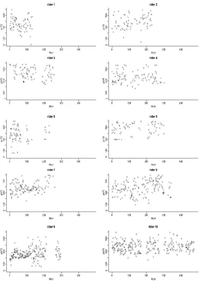
( ) (3.8) where is the ambient temperature in in session and is the time units into the session. To calculate the performance measure for each rider and for each session, a reference time and a reference temperature must be fixed. In our study, =1 hour and = 20 .Figure 3.12 shows an example of heart rate at lag 15 seconds versus power output with fitted line for rider 1 at a single session. The performance measures at ,
and for all sessions for each rider are presented in Figures 3.13, 3.14 and 3.15.
3.7
Summary
32
Table 3-3 Various percentiles of heart rate data for each rider
Rider 1 2 3 4 5 6 7 8 9 10
127 142 135 145 129 140 140 118 142 126 144 158 150 156 147 155 154 136 151 140 155 170 161 167 163 168 164 151 160 151
33
34
35
36
4
RELATING TRAINING TO PERFORMANCE
4.1
Introduction
In this chapter, the accumulation of training is related to the first of the performance measures described in the previous chapter, in order to determine the Banister model parameters. First, we describe the statistical distribution of our proposed performance measure. The performance measure itself is defined in section 3.6.2. This measure depends on the approximately linear relationship between power output and heart rate. Then we use the Banister model as a measure of training. These measures of training and performance are related to present a statistical model of training and performance. Through this, the Banister model parameters are estimated. The results of this model are discussed statistically and practically for each rider. Our methodology shows that the Banister model parameters can be estimated using data acquired in the field.
4.2
The Parameters of the Performance
–
Training Model
We relate the accumulated training effect (ATE) to our performance measure as follows: Firstly, we suppose that the relationship between performance and training is negatively linear. So the performance in session i, , is related to the accumulated training effect in session i, , as
( ) (4.1) with parameters , , and , the latter measuring the variability in the
performance-training relationship. The ATE was previously defined in chapter 3 by equation (3.4). Then, we obtain the estimated performance for each session for each rider which is defined from (3.6) in chapter 3 as
̂ ( ̂ ̂ ) ̂. This estimated performance is assumed to be distributed as
̂ ( ). (4.2) The variances ( =1,…,n) are the variability in the relationship between power output and heart rate; these variances must be estimated, n is the training session for a rider . To accomplish this, we use the delta method (Casella & Berger, 2002, p.240) as follows: Through the relationship between power output and heart rate given in equation (3.5), we can define power output for a session as:
37 Therefore
In the general form the delta method provides the variance of a function of parameter estimates:
[ ( ̂)] ∑ ∑ ( ̂ ̂ ).
In our case here, we have ( ) ( ) and
( ) so that
Hence, the variances ( =1,…,n)for each session can be obtained and ̂ for all as follows
̂
̂ { ̂ ( ̂ ) ̂ ̂ ( ̂) ( ) ̂ ( ̂) ̂ ̂ ( ̂ ̂ ) ̂ ( ̂ ̂) ̂ ̂ ( ̂ ̂)}
where and .
The final step in our method is, through (4.1) and (4.2), to write the model of training– performance as
̂ ( )
The parameters of this model , , , , and are estimated using the method of the maximum likelihood. Maximum likelihood estimation is considered as a preferred method of parameter estimation and is a fundamental tool for many statistical modelling techniques (Stuart et al., 1999). In this study, the estimation of the parameters is carried out in R (R Development Core Team, 2005).
This procedure is done to determine the values that maximise the log-likelihood function: ( ) ∑ ( ) ∑( ̂ ) ( )
38
Table 4-1 Estimated parameters with standard errors of the model for performance measure and =2 for each rider, with the t statistic and p value for the test of β=0.
R ider ̂ ( ̂ ) ̂ ( ̂ ) ̂ ( ̂ ) ̂ ( ̂
) ̂ ( ̂) t
1 12.2 3.5 78 61.1 9.8 1.9 139 6.4 -0.0027 0.0009 -3.00 0.00 2 3.1 1.9 5 2.1 0.7 0.2 160 4.1 -0.0406 0.0198 -2.05 0.02 3 12.3 6.1 78 87.3 9.3 6.6 140 5.6 -0.0015 0.0005 -3.00 0.00 4 2.4 1.6 137 28.4 44.2 10.8 139 2.8 -0.0034 0.0006 -5.00 0.00 5 23.4 3.5 184 103.2 0.2 1.5 156 6.2 -0.0026 0.0012 -2.17 0.02 6 0.2 1.6 182 88.1 17.0 2.3 156 4.7 -0.0024 0.0014 -1.71 0.04 7 7.1 1.3 175 118.6 0.5 2.1 146 3.9 -0.0016 0.0008 -2.00 0.02 8 2.1 1.2 62 25.4 32.1 11.7 122 2.3 -0.0030 0.0011 -2.73 0.00 9 3.2 0.8 7 2.1 3.3 0.9 145 2.2 -0.0128 0.0069 -1.86 0.03 10 2.4 0.7 166 40.7 33.1 11.1 130 2.1 -0.0013 0.0003 -4.30 0.00 Table 4-2 Estimated parameters with standard errors of the model for performance measure
and =2 for each rider, with the t statistic and p value for the test of β=0.
R ider ̂ ( ̂ ) ̂ ( ̂ ) ̂ ( ̂ ) ̂ ( ̂
) ̂ ( ̂) t
1 6.9 1.2 33 16.3 1.3 2.5 158 4.4 -0.0030 0.0014 -2.14 0.02 2 6.4 1.7 7 2.7 0.3 0.1 186 5.5 -0.0288 0.0126 -2.29 0.01 3 3.9 1.4 9 4.2 3.2 1.1 159 2.8 -0.0213 0.0127 -1.68 0.05 4 1.2 2.1 194 62.1 24.2 10.6 162 2.7 -0.0019 0.0005 -3.80 0.00 5 2.4 3.6 118 143.4 62.1 30.8 174 12.1 -0.0037 0.0021 -1.76 0.04 6 3.2 2.9 139 31.8 0.1 13.6 197 4.5 -0.0042 0.0009 -4.60 0.00 7 4.9 1.1 82 31.9 0.5 2.6 172 3.6 -0.0020 0.0008 -2.50 0.01 8 7.9 0.9 5 3.1 0.1 0.1 150 2.90 -0.0130 0.0088 -1.50 0.07 9 4.7 0.9 7 2.2 3.6 0.9 158 2.40 -0.0129 0.0071 -1.82 0.04 10 5.4 0.7 144 26.5 35.3 10.4 151 2.50 -0.0017 0.0004 -4.20 0.00
Table 4-3 Estimated parameters with standard errors of the model for performance measure when for each rider, with the t statistic and p value for the test of β=0.
R ider ̂ ( ̂ ) ̂ ( ̂ ) ̂ ( ̂ ) ̂ ( ̂ ) ̂ ( ̂
) ̂ ( ̂) t
39
Table 4-4 Estimated parameters with standard errors of the model for performance measure when for each rider, with the t statistic and p value for the test of β=0.
R ider ̂ ( ̂ ) ̂ ( ̂ ) ̂ ( ̂ ) ̂ ( ̂ ) ̂ ( ̂
) ̂ ( ̂) t
1 6.9 1.2 32 16.7 1.7 4.5 2.0 3.2 158 4.5 -0.0031 0.0015 -2.10 0.02 2 9.0 1.8 86 65.4 4.0 2.1 0.1 2.6 181 8.1 -0.0032 0.0017 -1.88 0.03 3 4.3 1.5 16 6.3 4.7 4.3 1.4 1.1 162 2.9 -0.0091 0.0047 -1.94 0.03 4 2.1 2.3 98 27.4 1.1 0.3 33.1 6.2 171 4.1 -0.0054 0.0029 -1.86 0.03 5 25 3.6 181 10.6 1.4 0.4 25.6 77.1 175 9.5 -0.0085 0.0073 -1.17 0.12 6 0.8 3.1 164 51.2 2.0 0.9 27.3 16.6 187 5.6 -0.0040 0.0018 -2.22 0.01 7 4.9 1.1 90 62.3 7.1 4.8 0.1 4.3 172 3.5 -0.0015 0.0008 -1.87 0.03 8 7.1 0.7 201 79.1 1.1 0.1 61.4 80.6 142 4.3 -0.0103 0.0041 -2.51 0.01 9 4.4 0.9 155 78.4 3.2 2.9 8.2 3.4 162 5.4 -0.0004 0.0002 -2.00 0.02 10 6.1 0.8 75 21.6 2.0 0.5 34.3 9.7 149 3.7 -0.0038 0.0018 -2.11 0.02
4.3
Statistical Discussion of the Training Effect
In this section, the relationship between the accumulated training effect and our proposed performance are discussed from a statistical perspective. This relationship is expected to be linearly negative. Therefore, we would like to reject the hypothesis in favour of . To test this hypothesis, we use T test at a significance level of 0.05 using ̂ ̂ ⁄ ( ( ̂)), where ( ̂) is the standard error for ̂. From Tables 4-1, 4-2, 4-3 and 4-4, we conclude that the relationship between training and performance is statistically significant at level 5% when ̂ . This relationship is negative for all riders ( < 0). However, in some riders, it can be observed that the value of the ̂ is greater than -1.64. For example, rider 8 for performance measure at =2, and rider 5 for performance measure when is free.
4.4
Practical Discussion of the Training Effect
The practical interpretation of the training effect for each rider is discussed in this section. To accomplish this, the changes in power output from the beginning of training until the point at which a rider has completed the optimal amount of training must be calculated. This is expressed as follows:
̂ ( ̂)
40
with percentiles of power output data and . These changes are greater or equal to 5% for all riders, excluding rider 5 at ( ), which his results may have been influenced by the multiple gaps in his data.
Table 4-5 The coefficients of the model between power output and heart rate from the last 60 days
Rider ̂ ( ) ̂ ( ) ̂ ( )
1 -102 (2.1) 2.66 (0.02) -0.00040 (0.000004) 2 -195 (2.5) 2.95 (0.02) -0.00008 (0.000040) 3 -35 (2.4) 1.94 (0.02) -0.00030 (0.000010) 4 59 (2.5) 1.51 (0.02) -0.00001 (0.000001) 5 -58 (2.1) 2.08 (0.02) -0.00010 (0.000008) 6 -248 (4.3) 3.89 (0.03) -0.00015 (0.000010) 7 -36 (3.1) 1.90 (0.03) -0.00019 (0.000010) 8 -220 (1.8) 3.35 (0.02) -0.00002 (0.000005) 9 -167 (2.9) 2.54 (0.02) -0.00008 (0.000007) 10 -142 (2.1) 2.79 (0.02) -0.00030 (0.000009)
Table 4-6Performance gain and the ATE change for each rider at performance measure and =2
Rider ̂ /
1 -0.0027 4166 30 225 0.13
2 -0.0406 801 96 235 0.41
3 -0.0015 3340 10 239 0.05
4 -0.0034 3455 14 213 0.07
5 -0.0026 13700 74 213 0.35
6 -0.0024 7541 70 293 0.24
7 -0.0016 10024 31 238 0.13
8 -0.0030 892 9 197 0.05
9 -0.0128 486 16 184 0.09
10 -0.0013 6992 25 208 0.12
Table 4-7 Performance gain and the ATE change for each rider at performance measure and =2
Rider ̂ /
1 -0.0030 3541 28 291 0.10
2 -0.0288 1252 106 307 0.35
3 -0.0213 501 21 291 0.07
4 -0.0019 7919 17 246 0.07
5 -0.0037 1794 12 280 0.05
6 -0.0042 8483 139 384 0.36
7 -0.0020 6808 26 323 0.08
8 -0.0130 807 35 274 0.13
9 -0.0129 478 16 214 0.08
41
Table 4-8 Performance gain and the ATE change for each rider at performance measure and is free with percentile of power output
Rider ̂ /
1 -0.0050 1579 21 225 0.09
2 -0.0400 799 94 235 0.40
3 -0.0062 882 11 239 0.04
4 -0.0129 1534 23 213 0.10
5 -0.0044 2244 21 213 0.09
6 -0.0035 2153 29 293 0.09
7 -0.0017 9321 30 238 0.13
8 -0.0039 980 13 197 0.07
9 -0.0003 15242 12 184 0.07
10 -0.0035 2614 26 208 0.13
Table 4-9 Performance gain and the ATE change for each rider at performance measure and is free with percentile of power output
Rider ̂ /
1 -0.0031 3433 28 291 0.10
2 -0.0032 6774 64 307 0.20
3 -0.0091 1315 23 291 0.08
4 -0.0054 3826 24 246 0.10
5 -0.0085 399 7 280 0.03
6 -0.0040 5738 89 384 0.23
7 -0.0015 7224 21 323 0.06
8 -0.0103 896 31 274 0.11
9 -0.0004 17829 18 214 0.08
10 -0.0038 2155 22 260 0.09
4.5
Discussion of Results
In this section, due to the individuality of the capacities of each of the riders, the findings are discussed statistically and practically for each rider from the results obtained.
For rider (1), significant relationships between the performance measures and the ATE are observed, as presented in Tables 4-1, 4-2, 4-3, and 4-4. Moreover, the training effect for this rider is practically significant in the practical sense for all cases and performance for this rider is increasing by about 13%, 10%, 9% and 10%, as this can be seen in Tables 4-6, 4-7, 4-8 and 4-9. Furthermore, the ATE decreases slightly after 50 days, as shown in Figures 4.1, 4.2 and 4.4.