INFORMATION BULLETIN ON VARIABLE STARS
Volume 63 Number 6256 DOI: 10.22444/IBVS.6256
Konkoly Observatory Budapest
10 December 2018 HU ISSN 0374 – 0676
PERIOD ANALYSIS, ROCHE MODELING AND ABSOLUTE PARAMETERS FOR AU Ser, AN OVERCONTACT BINARY SYSTEM
ALTON, K.B.1; NELSON, R.H2; TERRELL, D.3 1
Desert Bloom and UnderOak Observatories, 70 Summit Ave, Cedar Knolls, NJ, USA, email: [email protected]
2
Mountain Ash Observatory, 1393 Garvin Street, Prince George, BC, V2M 3Z1, Canada 3
Department of Space Studies, Southwest Research Institute, 1050 Walnut St., Suite 400, Boulder, CO 80302, USA
Abstract
CCD photometric data collected at UnderOak Observatory (UO) and Desert Bloom Observatory (DBO) in three bandpasses (B,V andIC) produced 10 new times of minimum for AU Ser which were used to revise the linear ephemeris. These results captured in 2011 and 2018 reinforced a longstanding observation that the shape of the light curve from this W UMa binary system (P=0.386497 d) is highly variable. Significantly skewed peaks and differences at maximum light were detected during quadrature which could only be simulated during Roche modeling by positioning a hot spot on the secondary star close to the neck between both constituents. Historically this system has been variously classified as an F8, G5 and K0 system; however, this study supports more recent reports that AU Ser is best described as spectral type K1V-K2V. A fresh assessment of eclipse time residuals over the past 80 years has provided additional insight regarding cyclical changes in orbital period experienced by this interesting variable star.
1
Introduction
The W UMa variable AU Ser was first discovered by Hoffmeister (1935), visually observed by Soloviev (1951) and photographically recorded by Huth (1964). Since 1972, at least four different studies have produced photoelectrically-derived light curves (Binnendijk 1972; Kennedy 1985; Li et al. 1992; Li et al. 1998). CCD photometric (V-mag) data for this system were also captured by the All Sky Automated Survey (ASAS) between 2003 and 2009 (Pojma´nski 2005). Two spectroscopic investigations of this system (Hrivnak 1993; Pribulla et al. 2009) produced radial velocity (RV) results critical to determining a mass ratio (q= 0.71±0.02) and total mass.
zone of a star. Light curves generated by Li et al. (1998) further highlight the challenge in modeling this overcontact binary and even proposed the existence of short period os-cillations at 0.0003 and 0.008 Hz. Period studies (Qian et al. 1999; G¨urol 2005, Amin 2015 and Nelson et al. 2016) from eclipse timings that extend as far back as 1936 have revealed secular changes over the past 80 years. An underlying sinusoidal relationship in the eclipse timing differences (ETD) led the most recent three investigators to propose a third body orbiting the binary pair. Various opinions abound, but there is a general consensus that the secular decrease in eclipse timings most likely results from mass trans-fer and that the cyclic light-time-effect (LiTE) originates from the gravitational influence of an unseen third star. Herein we report on the analysis of new multicolor (BV IC) LC
data acquired in 2011 and 2018 along with a retrospective analysis of all evaluable LCs from AU Ser that are available from the literature. Furthermore, fresh LiTE analyses supported by the addition of 10 new eclipse timings has resulted in the refinement of a period solution for a putative gravitationally-bound third body.
2
Data
The imaging apparatus used during 2011 at UnderOak Observatory (UO; NJ, USA) in-cluded a 0.28-m Schmidt-Cassegrain telescope with an SBIG ST-8XME CCD camera mounted at the Cassegrain focus. Additional time-series photometric observations were acquired in 2018 at Desert Bloom Observatory (DBO: Benson, AZ, USA) with an SBIG STT-1603ME CCD camera mounted at the Cassegrain focus of a 0.4-m catadioptric tele-scope. In both cases photometric B, V and IC filters manufactured to match the Bessell
prescription were used during each guided exposure (UO:75 s and DBO:60 s). Specifics regarding image acquisition, calibration, registration and reduction to catalog-based mag-nitudes (MPO Canopus) have been reported elsewhere for UO (Alton 2016) and DBO (Alton 2018). Roche type modeling was performed with the assistance of Binary Maker 3 (BM3; Bradstreet and Steelman 2002), WDwint56a (Nelson 2009), and PHOEBE 0.31a (Prˇsa and Zwitter 2005), the latter two of which employ the Wilson-Devinney (W-D) code (Wilson and Devinney 1971; Wilson 1979; Wilson 1990). Spatial renderings of AU Ser were also produced by BM3 once model fits were finalized. Times-of-minimum were cal-culated using the method of Kwee and van Woerden (1956).
3
Results
3.1 Photometry and Ephemerides
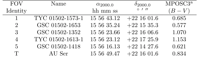
An ensemble of five stars in the same field-of-view with AU Ser (Fig. 1) was used to ultimately derive catalog-based magnitudes (Table 1). These stars exhibited no evidence of inherent variability (V and IC < 0.03 mag and B < 0.05 mag) beyond experimental
error over each imaging session. Photometric data in B (n=270), V (n=276), and IC
(n=284) were processed to generate bandpass specific LCs collected between 11 July 2011 and 22 July 2011 (Figs. 2 & 3). Additional photometric data acquired during a recent photometric campaign (29 May - 11 June 2018) inB (n=372),V (n=372) andIC(n=374),
were similarly folded by Fourier analysis (Figs. 2 & 3).
Table 1. FOV identity, name, astrometric coordinates and color index (B−V) for the target (AU Ser=T) and comparison stars (1-5) used for ensemble aperture photometry
FOV Name α2000.0 δ2000.0 MPOSC3a
Identity hh mm ss ◦ ′ ′′ (B−V)
1 TYC 01502-1573-1 15 56 43.12 +22 16 01.6 0.685 2 GSC 01502-1653 15 56 35.24 +22 15 35.3 0.577 3 GSC 01502-1352 15 56 23.66 +22 16 06.6 1.070 4 TYC 01502-1613-1 15 56 23.12 +22 17 25.9 1.153 5 GSC 01502-1418 15 56 16.13 +22 14 27.6 0.621
T AU Ser 15 56 49.47 +22 16 01.6 0.834
a: MPOSC3 is a hybrid catalog which includes a large subset of the Carlsberg Meridian Catalog (CMC-14) as well as from the Sloan Digital Sky Survey (Warner 2007).
Harris 1989) in MPO Canopus (2015) provided an identical period solution (0.386497 ± 0.000001d) for the multicolor data captured in 2011 and 2018. An updated linear ephemeris equation (1) based on the linear elements defined by Kreiner (2004) was calcu-lated using the last 7 years (Table 2) of published ET data:
Min I(Hel.) = 2458280.7899(14) + 0.3864965(1) E. (1)
Given the complex changes in orbital period observed for this system (see Section 3.6), new eclipse timings for AU Ser should be determined on a regular basis to maintain an accurate record about the behavior of this variable system.
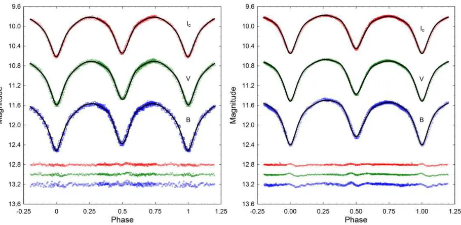
[image:3.595.117.483.424.669.2]Figure 2. Folded (P = 0.386497±0.000001 d) light curves (BV IC-mag) for AU Ser produced from
data collected in 2011 at UO (left) and during 2018 at DBO (right). Roche model fits using the W-D code were determined without the addition of a spot. For presentation convenience, the corresponding
residuals shown at the bottom are offset from zero.
Figure 3. Folded (P = 0.386497±0.000001 d) light curves (BV IC mag) for AU Ser produced from
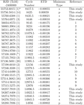
[image:4.595.74.529.458.680.2]Table 2. Eclipse time differences (ETD) between 2011 and 2018 calculated from published times of minima (ToM) for AU Ser along with ten new values reported for the first time in this study
HJD (ToM) Cycle ETD Minimum Reference
-2400000 Number Type
55753.6815 (1)a 8417.5 −0.00055 s This study
55756.5814 (14) 8425 0.00059 p This study 55760.6388 (1) 8435.5 −0.00021 s This study 55764.6971 (3) 8446 −0.00010 p This study
56034.8573 (1) 9145 −0.00175 p 1
56065.3904 (4) 9224 −0.00196 p 2
56511.4074 (2) 10378 −0.00318 p 3
56782.5374 (9) 11079.5 −0.00126 s 4
56783.5018 (7) 11082 −0.00310 p 4
56787.3675 (1) 11092 −0.00238 p 5
56787.3678 (1) 11092 −0.00207 p 6
56812.4894 (9) 11157 −0.00282 p 4
57084.9700 (1) 11862 −0.00303 p 7
57108.1609 (b) 11922 −0.00199 p 8
57135.7953 (3) 11993.5 −0.00217 s 7
57136.5691 (20) 11995.5 −0.00136 s 9
57198.6010 (2) 12156 −0.00237 p This study
57246.3338 (1) 12279.5 −0.00198 s 5
57414.6499 (3) 12715 −0.00555 p 10
57480.5515 (7) 12885.5 −0.00182 s 5
57514.3682 (16) 12973 −0.00366 p 9
57514.5613 (8) 12973.5 −0.00381 s 9
57515.5275 (8) 12976 −0.00386 p 9
58257.7919 (2) 14896.5 −0.00810 s This study 58267.8408 (1) 14922.5 −0.00817 s This study 58274.7979 (1) 14940.5 −0.00804 s This study 58276.7312 (1) 14945.5 −0.00720 s This study 58280.7886 (1) 14956 −0.00802 p This study
a: Throughout this paper tabulated uncertainty in least significant figure(s) provided within adjacent parentheses.
b: not reported;
3.2 Light Curve Behavior from 2011 and 2018
As is typical for overcontact binary systems, light curves from AU Ser (Figs. 2 & 3) exhibit minima which are separated by 0.5 phase (φ) and consistent with synchronous rotation in a circular orbit. Maximum light during the 2011 campaign was nearly equal (Max I ∼ Max II) within each bandpass; however, there is significant displacement whereby the brightest values occur after φ = 0.25 (+0.03) and before φ = 0.75 (-0.03). This effect is most obvious in B band and results in skewed peaks during quadrature. Similar behavior is observed with the 2018 light curves (Figs. 2 & 3), except that during this epoch Max I is notably brighter than Max II. It would appear that some kind of surface phenomenon distorts maximum light. Data from folded 2011 LCs B,V andIC mag) were
binned into equal phase intervals (0.002) to produce plots in which color index changes in B −V (Fig. 4: left) and V −IC (Fig. 4: right) were examined during each orbital phase. Deviation is quite remarkable suggesting that the localized effective temperature increased considerably during quadrature when the neck is maximally exposed.
Surface inhomogeneities have been associated with the presence of cool starspot(s), hot region(s), gas stream impact on either stellar partner, and/or other unknown mechanisms (Yakut and Eggleton 2005). As will be described in more detail in Section 3.4, positioning a hot spot on or near the neck region of the secondary star provided much improved Roche model solutions for the light curve asymmetry observed from 1969-2018. As mentioned earlier, Ka lu˙zny (1986) first proposed that a hot spot was responsible for the pronounced asymmetry observed in light curves captured in 1969 and 1970 by Binnendjik (1972). This is in contrast to Roche modeling (W-D) performed by G¨urol (2005) who concluded these LCs along with those collected in 1995 (Li et al. 1998) and 2003 (G¨urol 2005) were best fit with cool spots on the secondary. G¨urol (2005) did, however, show that simulated light curves collected in 1991 (Li et al. 1998) and 1992 (Li et al. 1998) benefited from hot spots on the secondary albeit not in the neck region. It should also be mentioned that G¨urol (2005) took an unorthodox approach by allowing A2, the reflection-coefficient of
the secondary, to freely vary during model optimization by differential corrections (DC). As a result the derived values were much larger (3.25–4.44) than the bolometric albedo value (0.5) usually assigned to systems with a convective envelope.
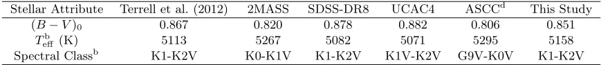
3.3 Effective Temperature
Color index (B−V) data from UO and five other surveys (Table 3) were corrected using the interstellar extinction (AV = 0.065; E(B-V) = 0.021 assuming R = 3.1) estimated
for targets within the Milky Way Galaxy according to Amˆores and L´epine (2005). The interstellar extinction model GALExtin1 requires the Galactic coordinates (l,b) and the
estimated distance in kpc. In this case the value for AV (0.065) corresponds to a target
located within 164 pc (see Section 3.5). By contrast the dust maps constructed by Schlegel et al. (1998) and updated by Schlafly and Finkbeiner (2011) determine extinction (AV =
0.172) based on total dust infrared emission in any given direction and not the extinction within a certain distance. In many cases the net effect for relatively close (<1 kpc) stellar objects within the Milky Way Galaxy is an overestimation of reddening. The mean result for intrinsic color, (B−V)0 = 0.859±0.021, which was adopted for subsequent Roche
modeling corresponds to an effective temperature of 5140 K (Pecaut and Mamajek 2013) and ranges in spectral class between K1V and K2V. The (V −IC)0 color index estimate (0.91±0.02) for the primary star taken at Min II when the secondary nearly reaches total
Table 3. Effective temperature of AU Ser based upon dereddened (B−V)a
data from various surveys and the present study
Stellar Attribute Terrell et al. (2012) 2MASS SDSS-DR8 UCAC4 ASCCd
This Study (B−V)0 0.867 0.820 0.878 0.882 0.806 0.851
Tb
eff (K) 5113 5267 5082 5071 5295 5158 Spectral Classb
K1-K2V K0-K1V K1-K2V K1V-K2V G9V-K0V K1-K2V a: E(B-V)= 0.021
b: Interpolated Teff and spectral class range estimated from Pecaut and Mamajek (2013)
c: Median value for (B−V)0 = 0.859 ±0.021;Teff1= 5140±125 K corresponds to spectral class K1V-K2V d: All-sky Combined Catalog of 2.5 million stars 3rd version (Kharchenko 2001)
eclipse is also consistent with a K1V-K2V spectral class (Pecaut and Mamajek 2013). Further support for our adopted Teff1 value comes from the Gaia DR2 database in which
the nominal Teff (5006 K) for this system is estimated to lie between 4761 and 5197 K
(Andrae et al. 2018).
3.4 Roche Modeling
3.4.1 Simultaneous LC and RV solutions
The program PHOEBE 0.31a (Prˇsa and Zwitter 2005) which features a user friendly in-terface to the WD2003 code (Wilson and Devinney 1971; Wilson 1979; Wilson 1990) was primarily used for initial Roche modeling of LC and RV data. Uncertainty estimates for each of the fitted parameters were ultimately derived using WDwint56a (Nelson 2009), a Windows front-end to the WD2003 source code. In both cases ”Mode 3” (Wilson and Leung 1977) designated for overcontact binary systems was selected for fitting while each curve was weighted based upon observational scatter. Bolometric albedo (A1,2=0.5) and
gravity darkening coefficients (g1,2 = 0.32) for stars with convective envelopes were
re-spectively assigned according to Ruci´nski (1969) and Lucy (1967). New logarithmic limb darkening coefficients (x1, x2, y1, y2) were interpolated (Van Hamme 1993) following any
change in the effective temperature for the secondary (Teff2) star. The effective
temper-ature of the more massive and brighter primary constituent was fixed (Teff1 = 5140 K).
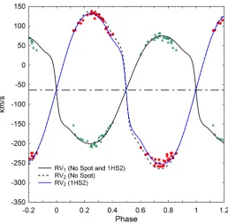
RV data published by Pribulla et al. (2009) were also used to further refine a LC so-lution for AU Ser. These data, collected in 2008, were obtained using the broadening functions extracted from the Mg I triplet region (5184 ˚A) located within the V bandpass. As appropriate, RV data were modeled (WDwint56a) with LC data to produce the best simultaneous fits using multiple parameter subsets during DC iterations. The correspond-ing parameters which were varied included the center-of-mass velocity (V γ), semi-major axis (SMA), mass ratio (q), surface potential (Ω1 = Ω2), inclination (i) and Teff2.
Preliminary Roche modeling attempts had revealed that the addition of a hot spot in the neck region of the secondary star was critical to successfully obtaining a good fit of the LC data. It should also be pointed out that the RV solution for the secondary (RV2)
well-sampled LC (V mag) collected in 1991 (Li et al. 1992) is the closest match ((Max I - Max II) = −0.026) to that captured during the 2008 survey. Both LCs (1991 and 2008) produced similar results (q= 0.684±0.006 vs. 0.699±0.006) when simultaneously modeled with the 2008 RV data. The mean mass ratio value (0.692±0.006) calculated from the 1991 and 2008 LCs was utilized for subsequent Roche modeling and fixed during DC iterations.
Figure 4. Simultaneous radial velocity (RV) solution for AU Ser without and with a single hot spot in the neck region of the secondary star (1HS2).
3.4.2 Light Curves from 2011 and 2018
As mentioned previously, Roche modeling was constrained using the mass ratio (q = 0.692±0.006) determined after simultaneously modeling RV and LC data (Section 3.4.1). This value is slightly lower than that (qsp = 0.71) determined using RV data alone by
Hrivnak (1993) and Pribulla et al. (2009). All other parameters except forTeff1,A1,2 and
g1,2 were allowed to vary during DC iterations. Multi-color parameter values and results
from modeling the 2011 and 2018 LCs are found in Table 5. Corresponding unspotted (Fig. 2) simulations reveal the poor model fit during quadrature which could be signifi-cantly improved by the addition of a hot spot near the neck region shared by both stars (Fig. 3).
The fill-out parameter (f) which corresponds to the degree of overcontact between each star was calculated (Eq. 2) according to Kallrath and Milone (1997):
f = (Ωinner−Ω1,2)/(Ωinner−Ωouter), (2)
where Ωouter is the outer critical Roche equipotential, Ωinner is the value for the inner
critical Roche equipotential and Ω1,2 denotes the common envelope surface potential for
[image:9.595.80.531.274.666.2]the binary system. An interesting finding (Table 6) is that the fill-out factor varies substantially (1.5 - 27.3%). One possibility considered was an association between the fill-out factor and the O’Connell effect, however, this proved not to be the case. Attempts to model the LC data from 2018 (f = 4%) as a detached (Mode 2) and semi-detached (Mode 5) system never approached the best Roche lobe fits achieved when AU Ser was considered an overcontact system (Mode 3).
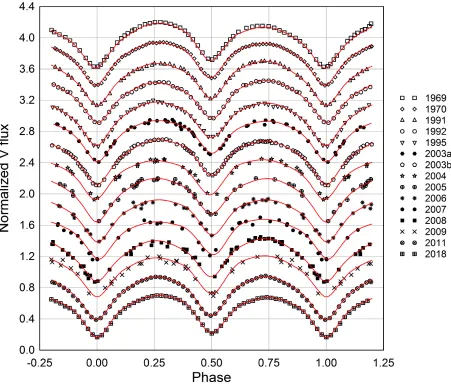
Figure 5. Folded (P = 0.386497±0.000001 d) light curves for AU Ser produced from publishedV mag data collected between 1969 to 2009 as well as new results reported herein from 2011 and 2018. In each case, Roche modeling with the W-D code required the addition of a single hot spot in the neck region of
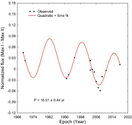
Figure 6. LC variations in Max I-Max II between 1969 and 2018. Differences were fit to a quadratic + sinusoidal expression. The results suggested that there is a∼16.5 yr cycle that may be associated with
the O’Connell effect.
Table 4. Differences (±SD) in normalized V-flux relative to Max I Year Max I-Min I Max I-Min II Max I-Max II 19691 0.572 (6) 0.479 (7) 0.045 (6)
19701 0.561 (6) 0.465 (8) 0.023 (6)
19912 0.562 (8) 0.478 (6) −0.026 (8)
19922 0.540 (9) 0.484 (6) −0.016 (7)
19953 0.544 (7) 0.423 (9) 0.031 (4)
2003a4 0.586 (6) 0.458 (4) 0.023 (4)
2003b5 0.527 (9) 0.436 (6) −0.003 (7)
20045 0.502 (13) 0.463 (12) −0.001 (8) 20055 0.564 (26) 0.455 (11) −0.008 (7)
20065 0.492 (11) 0.404 (11) −0.034 (8)
20075 0.480 (10) 0.422 (16) −0.051 (5)
20085 0.500 (8) 0.425 (9) −0.059 (5)
20095 0.447 (13) 0.453 (15) −0.021 (6)
20116 0.554 (7) 0.502 (6) −0.004 (8)
20186 0.496 (6) 0.462 (6) 0.012 (6)
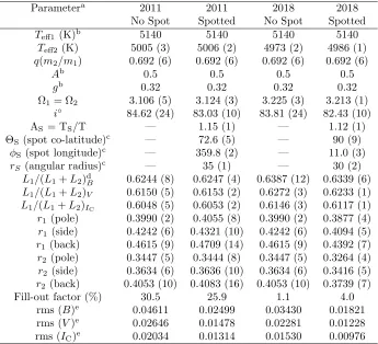
[image:10.595.174.424.520.713.2]Table 5. Light curve parameters employed for Roche modeling and derived geometric elements for the AU Ser light curves captured in 2011 and 2018
Parametera 2011 2011 2018 2018
No Spot Spotted No Spot Spotted
Teff1 (K)b 5140 5140 5140 5140
Teff2 (K) 5005 (3) 5006 (2) 4973 (2) 4986 (1)
q(m2/m1) 0.692 (6) 0.692 (6) 0.692 (6) 0.692 (6)
Ab 0.5 0.5 0.5 0.5
gb 0.32 0.32 0.32 0.32
Ω1= Ω2 3.106 (5) 3.124 (3) 3.225 (3) 3.213 (1)
i◦ 84.62 (24) 83.03 (10) 83.81 (24) 82.43 (10)
AS= TS/T — 1.15 (1) — 1.12 (1)
ΘS(spot co-latitude)c — 72.6 (5) — 90 (9)
φS(spot longitude)c — 359.8 (2) — 11.0 (3)
rS (angular radius)c — 35 (1) — 30 (2)
L1/(L1+L2)dB 0.6244 (8) 0.6247 (4) 0.6387 (12) 0.6339 (6)
L1/(L1+L2)V 0.6150 (5) 0.6153 (2) 0.6272 (3) 0.6233 (1)
L1/(L1+L2)IC 0.6048 (5) 0.6053 (2) 0.6146 (3) 0.6117 (1) r1 (pole) 0.3990 (2) 0.4055 (8) 0.3990 (2) 0.3877 (4)
r1 (side) 0.4242 (6) 0.4321 (10) 0.4242 (6) 0.4094 (5)
r1(back) 0.4615 (9) 0.4709 (14) 0.4615 (9) 0.4392 (7)
r2 (pole) 0.3447 (5) 0.3444 (8) 0.3447 (5) 0.3264 (4)
r2 (side) 0.3634 (6) 0.3636 (10) 0.3634 (6) 0.3416 (5)
r2(back) 0.4053 (10) 0.4083 (16) 0.4053 (10) 0.3739 (7)
Fill-out factor (%) 30.5 25.9 1.1 4.0
rms (B)e 0.04611 0.02499 0.03430 0.01821
rms (V)e 0.02646 0.01478 0.02281 0.01228
rms (IC)e 0.02034 0.01314 0.01530 0.00976
a: All error estimates forTeff2,q, Ω1,2,AS, ΘS, φS,rS,r1,2,L1from WDwint56a (Nelson 2009)
b: Fixed during DC
c: Secondary spot temperature, location and size parameters in degrees
d: Bandpass dependent fractional luminosity;L1 andL2refer to scaled luminosities of the primary
3.4.3 Retrospective analysis of LCs from 1969-2009
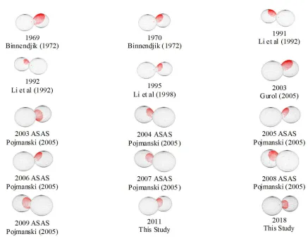
W-D modeling (V mag) of the six previously published LCs (Binnendjik 1972; Li et al. 1992; Li et al. 1998; G¨urol 2005) was performed with and without a hot spot located near the neck region in a manner similar to that previously described for the 2011 and 2018 data. In addition, sparsely sampled ASAS survey data (V mag) collected between 2003 and 2009 (Pojma´nski et al. 2005) were phased to produce yearly LCs (Fig. 6) using the ANOVA routine (Schwarzenberg-Czerny 1996) in Peranso 2.5 (Paunzen and Vanmunster 2016). Only the spotted solutions from this retrospective analysis are included herein. Roche modeling of the LCs generated during this period of time provided additional information to chronicle the behavior of AU Ser over a longer period of time than was available to G¨urol (2005). Relative V-flux levels at Min I, Min II, Max I and Max II were estimated using polynomial fits near each LC region of interest. A positive OConnell effect (Max I > Max II) was observed in 1969, 1970, 1995, 2003a and 2018, whereas Max II >
Max I in 1991, 1992, and between 2005-2009. LCs from 2003b, 2004 and 2011 did not exhibit any meaningful (≤0.004) differences in maximum light (Table 4). It should be noted that photometric data captured by G¨urol (2005) in 2003 occurred between 22 July and 26 Aug 2003, whereas the majority (80%) of the data during the ASAS survey were acquired before 22 July 2003. This may explain differences in the modeling results (2003a vs. 2003b).
A quadratic + sinusoidal fit (Fig. 7) of flux normalized Max I - Max II values over time (1969-2011) uncovered a periodic change (16.51±0.44 yr) in the LCs. G¨urol (2005) performed a similar analysis but over a shorter time frame (1969-2003) and arrived at a different conclusion which suggested the most probable period for flux variation relative to Max I ranged between 32 and 35 yr. Upon further examination, one finds that G¨urol (2005) proposed two other possible solutions at 8.9 and 17.3 yr. It is not hard to imagine period harmonics which are simple multiples in the ratio 8.5:17:34. The middle value closely approximates the more robust period estimate from this study and indicates that flux change relative to that observed at Max I occurred nearly every 17 yr and corresponds to the transition from a positive to negative O’Connell effect. Furthermore, assessment of the LCs and each corresponding Roche model fit (Table 6) offer compelling evidence for persistent feature(s) on AU Ser that skew maximum light to occur afterφ = 0.25 and then before φ = 0.75; the best fits were consistently achieved by positioning a hot spot on or near the neck region of the secondary star.
As depicted in Figure 8, spatial models of AU Ser showing the sequence of hot spot locations were rendered with BM3 using the physical and geometric elements determined from all LCs investigated herein. As might be expected, the longitudinal position of the hot spot relative to the neck center (0◦
hot spot would be maximally exposed.
IB
V
S
6
2
5
[image:14.595.72.767.228.339.2]6
Table 6. Light curve (V mag) parameters employed for Roche modeling (spotted) and derived geometric elements from AU Ser light curves captured between 1969 and 2018.
Parameter 19691
19701
19912
19922
19953
2003a4
2003b5
20045
20055
20065
20075
20085
20095
20116
20186 Teff1(K)
b
5140 5140 5140 5140 5140 5140 5140 5140 5140 5140 5140 5140 5140 5140 5140
Teff1(K) 4907(3) 4896(2) 4942(4) 4991(5) 4875(6) 4863(4) 4896(7) 4969(9) 4882(11) 4916(12) 4954(12) 4998(24) 5054(13) 5014(1) 4986(1) q(m2/m1) 0.692(6) 0.692(6) 0.684(6) 0.692(6) 0.692(6) 0.692(6) 0.692(6) 0.692(6) 0.692(6) 0.692(6) 0.692(6) 0.699(6) 0.692(6) 0.692(6) 0.692(6)
Ab
0.5 0.5 0.5 0.5 0.5 0.5 0.5 0.5 0.5 0.5 0.5 0.5 0.5 0.5 0.5
gb
0.32 0.32 0.32 0.32 0.32 0.32 0.32 0.32 0.32 0.32 0.32 0.32 0.32 0.32 0.32
Ω1,2 3.18(1) 3.19(1) 3.12(1) 3.16(1) 3.16(1) 3.18(1) 3.23(1) 3.22(1) 3.17(2) 3.19(2) 3.21(2) 3.19(2) 3.19(3) 3.13(3) 3.21(1)
i◦ 82.1(2) 82.0(1) 82.2(1) 81.5(3) 83.0(4) 83.2(2) 82.0(4) 81.0(1) 82.3(7) 81.2(8) 81.3(7) 82.7(1.8) 80.2(1.1) 82.8(1) 82.4(1)
AS=TS/T 1.11(1) 1.16(1) 1.17(1) 1.19(1) 1.11(1) 1.13(1) 1.14(1) 1.11(1) 1.11(1) 1.14(1) 1.15(2) 1.12(1) 1.12(1) 1.14(1) 1.12(1)
ΘS(co-lat.) c
49.6 (1.3) 59.6 (1.3) 50 (12) 65 (3) 70 (7) 46.2 (2) 19.6 (1) 70 (4) 65 (15) 62 (5) 56 (18) 59 (12) 79.5 (7.3) 71.1 (1) 90 (1) φS(long.)
c
18.5 (1.1) 4.2 (4) 352 (3) 350 (1) 5 (2) 6 (1) 6 (2) 355 (4) 2(5) 0 (3) 345 (5) 350 (6) 350 (6) 0(1) 11 (1)
rS (radius) c
60.1 (6) 37.3 (2) 40 (1) 25 (1) 35 (1) 48 (1) 48 (1) 33.8 (1.6) 34 (3) 35 (8) 28 (3) 36 (2) 36 (2) 35 (1) 30 (1)
Fill-out (%) 12.9 10.4 24.4 15 17 13 5.3 1.5 13.7 10.4 10.0 27.3 5.8 25.7 4
1. Binnendijk 1970; 2. Li et al. 1992; 3. Li et al. 1998; 4. G¨urol 2005; 5. Pojma´nski et al. 2005; 6. This study a: All error estimates forTef f2,q, Ω1,2,AS, ΘS,φS,rS from WDwint56a (Nelson 2009)
b: Values fixed during DC
Table 7. Mean absolute parameters (±SD) for AU Ser using results from the simultaneous (LC and RV) Roche model fit ofV mag data from 1991 and 2008.
Parameter Primary Secondary Mass (M⊙) 0.85 (3) 0.59 (2)
Radius (R⊙) 1.04 (1) 0.88 (1)
a(R⊙) 2.52 (3) —
Luminosity (L⊙) 0.675 (13) 0.427 (9)
Mbol 5.177 (22) 5.675 (22)
log(g) 4.336 (16) 4.323 (16)
3.5 Absolute Parameters
Absolute parameters (Table 7) were derived for each star in this A-type W UMa binary system using results from the best fit spotted model simulations from 1991 and 2008. Aside from a spectroscopic mass ratio (qsp), another critical piece of information supplied
by an RV experiment is the determination of the orbital speeds (v1r +v2r) whereby the
total mass can be readily calculated according to Eq. 3 when the orbital inclination is also known:
(m1+m2) sin3i= (P/2πG)(v1r+v2r)3. (3)
In this case from the mean simultaneous fit of LC and RV data (1991 and 2008),
K1 = 135.2±1.1 km/s ,K2 = 195.5±1.8 km/s,Vγ =−63.8±0.68 km/s andi= 82.5±1.8◦.
The total mass of the system was determined to be 1.44±0.05M⊙ so it follows that since
q = 0.692 ±0.006 then the primary mass = 0.85 ±0.03 M⊙ and secondary mass = 0.59±0.02M⊙.
The semi-major axis,a(R⊙) = 2.52±0.03, was calculated according to Newton’s version (Eq. 4) of Keplers third law where:
a3 =G×P2(M1 +M2)/4π2. (4)
The effective radii of each Roche lobe (RL) can be calculated to within an error of 1%
over the entire range of mass ratios (0< q < ∞) according to the expression (5) derived by Eggleton (1983):
rL = (0.49q(2/3))/(0.6q(2/3)+ ln(1 +q(1/3))) (5)
from which values for r1 (0.4112 ± 0.0005) and r2 (0.3475 ± 0.0005) were respectively
determined for the primary and secondary stars. Since the semi-major axis and the volume radii are known, one can calculate the solar radii for both binary constituents where R1
= a × r1 = 1.04± 0.01 R⊙ and R2 = a ×r2 = 0.88 ± 0.01 R⊙.
The bolometric magnitudes (Mbol1,2) and luminosity in solar units (L⊙) for the primary
(L1) and secondary stars (L2) were calculated from well known relationships for bolometric
magnitude (Eq. 6) and luminosity (Eq. 7) where:
Mbol1,2 = 4.75−5 log(R1,2/R⊙)−10 log(T1,2/T⊙) (6)
and
L1,2 = (R1,2/R⊙)2(T1,2/T⊙)4. (7)
Pooling the results for Tef f2 across all LCs (1991-2018) leads to a mean value of 4943±
and secondary are 0.675±0.013 and 0.427 ±0.020, respectively. Bolometric magnitudes were calculated to be Mbol1 = 5.127 ±0.009 and Mbol2 = 5.691 ±0.052. Combining
the bolometric magnitudes resulted in an absolute value (MV = 4.663 ± 0.009) when
adjusted with the bolometric correction (BC= −0.272) interpolated from Pecaut and Mamajek (2013). Substituting into the Eq. 8, the distance modulus:
d(pc) = 10((m−MV)−AV+5)/5), (8)
wherem=Vavg(10.71±0.01) and AV = 0.065 leads to an estimated distance of 171±2 pc
to AU Ser which is 5% higher than that (164±1 pc) calculated directly from parallax data recently included in the Gaia DR2 release (Brown et al. 2018). Although not unreasonable, this discrepancy may result from the use of MPOSC3-catalog based magnitudes rather than determining values from absolute photometry with reference star field standards.
3.6 Period analyses from eclipse time differences
Over the years there have been many period studies of this system. Kennedy (1985) was the first to suggest that changes had occurred in the eclipse timing differences (ETDs) for AU Ser. Qian et al. (1999) performed the first systematic examination of period and light time variations for this system and noted that the orbital period suddenly decreased between 1987 and 1988. They suggested there might be a connection between the light curve asymmetries and sudden changes in the orbital period. The next detailed analysis of the ETDs was conducted by G¨urol (2005) in which he modeled the residuals over time with a quadratic plus sinusoidal equation and subsequently dismissed the notion of a sudden period change. Furthermore G¨urol (2005) proposed that the predominant cyclic behavior with a period of about 94 yr was most likely associated with the light-time-effect (LiTE) caused by an invisible but gravitationally bound third star.
A case, albeit somewhat less convincing, can be made which argues against the presence of a gravitationally-bound third body. It should be noted that during our Roche modeling,
l3, the third light parameter, was not significantly different from zero when allowed to
freely vary during iterative DC. This implies that a putative gravitational partner in this system is either too small to detect during simulations of the observed light curve data or that some other phenomena are responsible for the ∼94 yr periodicity in the eclipse timing residuals. Assuming that the putative third body is still on the main sequence its absolute luminosity can be estimated according to the mass-luminosity relationship where
L∼M3.5. The fractional luminosity of the third constituent (L
3) can be calculated from
the expression (Eq. 9):
L3(%) = (100×M33,.min5 )/(L1+L2+M33,.min5 ) (9)
where M3 is the minimum mass determined when i = 90◦ and L1 and L2 are the
lu-minosities in solar units (L⊙) determined for the primary and secondary stars (Table 7).
Comparisons among third body solutions proposed by G¨urol (2005), Amin (2015), Nelson et al. (2016) and this study are summarized in Table 8. According to our LiTE modeling, the luminosity contributed by a third body (L3 ∼1.2%) whereM3 = 0.293 M⊙
would be challenging to detect photometrically. However, the minimum mass estimates for a third body reported (Table 8) by Amin (2015) and G¨urol (2005) would have resulted in even greater contributions (L3 >6%) to the total luminosity of the system. According
from an RV study in which Pribulla et al. (2009) did not see spectroscopic evidence for a third body in the broadening functions. It is clear that additional high-precision photometric and spectroscopic data will be necessary to fully tease out the effect(s) which lead to episodic changes in the eclipse timings for AU Ser.
Amin (2015) and Nelson et al. (2016) re-examined the period behavior of AU Ser using ETD data gathered between 1936 and 2015. Modeling efforts by Amin (2015) which included 39 new minima times led to values for a putative third body which contrast sharply with the period (P3) and semi-amplitude (A) reported by G¨urol (2005) and Nelson
et al. (2016). There was, however, general concurrence between Amin (2015) and G¨urol (2005) that the mechanism for a light-time effect was probably not due to cycles in magnetic activity attributed to Applegate (1992). This is further supported using an empirical relationship (Eq. 10) between the length of orbital period modulation and angular velocity (ω = 2π/Porb) that was developed by Lanza and Rodon`o (1999):
logPmod[y] = 0.018−0.36×log (2π(Porb[s])). (10)
In this case any period modulation resulting from a change in the gravitational quadru-pole moment would probably be closer to 23 yr for AU Ser, not the longer periods (P3 >
42 yr) proposed by G¨urol (2005) and Amin (2015). Significant differences in the quadratic coefficient were reported depending upon whether or not visual (vis) and photographic (pg) data were included in the analyses. This disparity points out the vagaries associated with period change and mass transfer analysis from eclipse timing residuals; other factors contributing to error are discussed in depth in a series of papers by Nelson et al. (2014; 2015; 2016). Ironically in Nelson et al. (2016), several widely different LiTE solutions emerged: A1 (an update to the analysis of G¨urol (2005) but using LiTE analysis in which
P3 = 29.9 yr),B1(another update to G¨urol 2005 whereP3 = 96.4 yr), and finally a new fit,
solution C (P3= 38.6 yr). Nelson et al. (2016) concluded that it was ”problematic which
solution to choose”; however they favored solution A1. Here again it was evident with
our fresh analysis which includes ETs reported by G¨urol (2005) and Amin (2015) and 10 new ETs from this study, that many early pg and vis eclipse timings identified as outliers in Fig. 10 seemingly describe a completely different pattern than all the others derived from ccd and photoelectric (pe) analyses. Removal of these data from consideration was not taken lightly, however, as it became very clear after multiple model iterations, their inclusion made it impossible to properly simulate the orbital period variability of AU Ser after 1969. This would severely limit the ability to predict future behavior of AU Ser and thus derive a robust hypothesis for the underlying sinusoidal-like variations in the orbital period. Data included in all subsequent (1969-2018) curve fitting were weighted in the ratio 0.04:1:1 (vis:pe:ccd).
Stepping back for a moment to first principles, shifts in the times of minimum light under the influence of a third body orbiting a binary system can be evaluated according to the generalized expression (Eq. 11):
(ETD)f itted =c0+c1E+c2E2+τ, (11)
where c0, c1 and c2 are constants, E = cycle or epoch number, and τ = time difference
due to orbital motion, an expression derived by Irwin (1952; 1959). Ignoring the last term (τ=0) for the moment, initial curve fitting (scaled Levenberg-Marquardt algorithm) revealed a quadratic coefficient (c2 ≈ −5.0×10⁻¹¹) that is less than zero (downwardly
momentum loss (AML) due to magnetic stellar wind. Ideally when AML dominates the net effect is a decreasing orbital period whereas the opposite is observed with conserva-tive mass transfer from the secondary to the primary star. Notably, residuals from the quadratic model fit also describe an underlying sinusoidal-like variation in the orbital period. As long as this sinusoidal curve appears symmetrical as suggested in the middle panel of Fig. 10, this behavior can be fit in its simplest form using a quadratic formula (Eq. 12) modulated with a sine term (τ) such that:
(ETD)fitted =c0+c1E+c2E2+c3sin(c4E+c5) (12)
where c0, c1 and c2 are constants, E = cycle number, and τ = time difference due to
orbital motion. This simplified light-time effect (LiTE) analysis using a scaled Levenberg-Marquardt (L-M) algorithm assumes that the putative third body revolves about a com-mon gravitational center in a circular orbit (e=0). The amplitude of the oscillation, as defined by the coefficient of the sine term (c3), was determined to be 0.0116±0.0003 d
while the period of the sinusoidal oscillations was calculated (P3 = 31.2±0.3 yr) according
to the expression (Eq. 13):
P3 = 2πP/ω , (13)
whereω, the angular frequency, is defined by the coefficient c4 (0.000213±0.000004) and
P is the orbital period of the binary pair in days. Cyclic changes of eclipse timings may result from the gravitational influence of unseen companion(s) and/or periodic changes in the magnetic activity of either binary constituent. It has been well documented that a sig-nificant percentage (>50%) of overcontact binaries exist as multiple systems (Pribulla et al. 2006; D’Angelo et al. 2006). Additional analyses including the associated parameters in the LiTE equation (Irwin 1952; 1959) were derived using the Solver routine in an Excel spreadsheet described by Nelson et al. (2016). These parameters include: P3 (orbital
pe-riod of star 3 and the 1-2 pair about their common center of mass), e (orbital eccentricity),
ω (argument of periastron), t3 (time of periastron passage) and the semi-amplitude (A)
of the light-time effect. The semi-amplitude is further defined as A = a12sin(i3)×c−1
wherea12= semi-major axis of the 1-2 pair’s orbit about the center of mass of the 3-star
system, i3 = orbital inclination of the 3-star system, and c = speed of light. These five
parameters, as well as the coefficients c0, c1, and c2 from Eq. 12 add up to a total of eight
variables which are factored into LiTE modeling. It was apparent from our simplified L-M solution (P3 = 31.2±0.3 yr) which included 10 new times-of-minima (Table 8) that
period (P3) solutions A1 (29.8 yr) and A2 (29.4 yr) from Nelson et al. (2016) were very
close. We repeated this simplest solution which fixes the third body with a circular orbit (e=0) and another where e is allowed to vary using the aforementioned eight parameter Excel Solver routine to optimize the LiTE fit. These two analyses produced similar results when comparing the root mean square errors (Table 8). The latter solution in which a putative third body revolves in a somewhat eccentric orbit (e= 0.168) appears to offer a slightly improved fit but at the expense of an increased error estimate forP3 (31.36±1.18
vs. 31.49±0.40 yr). Nonetheless, considering an improbably stable circular orbit for a circumbinary star, we arrive at a preferred solution in which the orbit is slightly elliptical (e = 0.168±0.023). Thereafter it was possible to subtract out the LiTE component of the ETD values leaving, in this case, a parabolic relationship with quadratic constant c2 =−6.19(20)×10−11 d (Fig. 10). Assuming that the secular decrease in orbital period
is associated with mass loss from the primary to the secondary, then a period rate loss (dP/dt=−1.17(4)×10−7 d/yr) can be estimated from Eq. 14:
Table 8. Putative period change, mass loss and third-body solution to the light-time effect observed from changes in AU Ser eclipse timings
Parameter Units G¨urol (2005) Amin (2015) Nelson et al. This study This study (2016)
t0 HJDa 44722.4515 44722.4683 (14) 44722.4472 44722.4725 44722.4725
t3 (init, epoch) [d] 10023.9468 10857 (533) — 10176 (2666)
P3 (period) [yr] 94.15 43 (3) 29.8 (5) 31.49 (40) 31.36 (1.18) A (Amplitude) [d] 0.0355 0.0197 (16) 0.0110 (3) 0.0109 (2) 0.0116 (4)
e (eccentricity) 0.48 0.52 (12) 0 0 0.168 (23)
ω, arg. periast. ◦ 147.7 — — — 163.7 (20.5)
a12sin(i) [AU] — 3.66 (30) 1.90 (5) 1.89 (3) 2.01 (8)
f(m3) M⊙ 0.034199 0.02662 (13) 0.0077 (5) 0.0068 (4) 0.0082 (14)
M3 (i=90◦) M⊙ 0.53 0.475 (1) — 0.271 0.293
M3 (i=60◦) M⊙ — 0.564 (1) — 0.319 0.342
M3 (i=30◦) M⊙ — 1.153 (3) — 0.612 0.661
c2 (Quad. coeff.) ×10−11 −
7.29 −4.69 −6.8 (3) −6.28 (8) −6.19 (20)
dP/dt 10−7
d/yr −1.378 −0.887 — −1.19 (1) −1.17 (4)
dM1/dt 10−7M⊙/yr −2.598 — — −1.95 (8) −1.93 (10)
rssb
0.000643433 0.000612608
a: HJD-24000000
b: Residual Sum of Squares (rss)
Finally, the rate of conservative mass transfer was calculated using Eq. 15:
dM/dt=M1M2/(3P(M1−M2))dP/dt, (15)
where M1 is the mass of the primary star in solar units, M2 is the mass of the secondary
star in solar units, and P is the orbital period of binary pair. Accordingly, the mass-transfer rate (dM1/dt) for AU Ser was estimated to be −1.93(10)×10−7M⊙/yr.
4
Conclusions
Reported herein are the first BV IC CCD-based light curves for AU Ser which have also
produced 10 new times of minimum for this A-type W UMa binary system. Evidence from this study and other surveys suggested that the effective temperature of the primary star was ∼ 5140 K which corresponds to a spectral class range between K1V and K2V. During Roche modeling with the W-D code, a spotted solution was necessary since all evaluable LCs from 1969 to 2018 exhibited asymmetry with regard to intensity and/or peak skewness during quadrature (maximum light was displaced afterφ= 0.25 and before
φ = 0.75). Positioning a single hot spot on the secondary near the neck between both stars produced the best Roche model fits. The relative location of the secondary hot spot corresponded to cyclical changes (∼ 16.5 yr) which appeared to be associated with the so-called ”O’Connell effect”. Regression analyses performed using ETDs indicate that the orbital period for AU Ser has been decreasing at a rate of ∼ 1.18×10⁻⁷
d yr−1
. This secular change in orbital period may be related to mass transfer from the primary onto the secondary and is consistent with the appearance of a persistent hot spot in the neck region of the secondary star. LiTE analysis on a subset of time-of-minimum observations spanning the last 49 years uncovered a sinusoidal-like variation (P3 ∼ 31.36 yr) in the
Figure 8. Preferred LiTE solution (P3= 31.36±1.2 yr) incorporating 10 new eclipse timings for
AU Ser. The top panel includes all eclipse time differences (ETD1) however the model fit does not
include those labeled as ”Outliers = *”. The bottom panel shows the residuals (ETD2) remaining from
magnetic activity) cannot be completely discounted. As is often the case with complex behaviors uncovered by analyzing secular changes in overcontact binary systems, many more years of data will likely be required to confirm the true nature of periodic variation observed in the eclipse timings.
Acknowledgements: This research has made use of the SIMBAD database, operated
at Centre de Donnes astronomiques de Strasbourg, France, the Northern Sky Variability Survey hosted by the Los Alamos National Laboratory and the International Variable Star Index maintained by the AAVSO. The diligence and dedication shown by all associated with these organizations is very much appreciated. We are indebted to the many observers who have published a wealth of eclipse timing data for AU Ser over the past 80+ years. This work has also made use of data from the European Space Agency (ESA) mission Gaia. This research did not receive any grant from funding agencies in the public, commercial, or not-for-profit sectors. In addition, we gratefully acknowledge the insightful comments from Prof. Robert Wilson and the careful review and commentary from an anonymous referee.
References:
Alton, K.B. 2016, JAAVSO, 44, 87 Alton, K.B. 2018, IBVS,63, 6241 DOI
Amin, S.M. 2015,J. Korean Astron. Soc.,48, 1
Amˆores, E.B. and L´epine, J.R.D. 2005,AJ,130, 659 DOI
Andrae, R., Fouesneau, M., Creevey, O., et al. 2018,A&A, 616, A8 DOI Applegate, J. 1992, ApJ, 385, 621 DOI
Binnendijk, L. 1972, AJ, 77, 603 DOI
Bradstreet, D.H. and Steelman D.P. 2002,Bull. A.A.S., 34, 1224
Brown, A.G.A., Vallenari, A., Prusti, T., et al. 2018, A&A, 616, A1 DOI D’Angelo, C., van Kerkwijk, M.H., Ruci´nski, S.M. 2006, AJ, 132, 650 Diethelm, R. 2012,IBVS, 61, 6029
Djuraˇsevi´c, G. 1992, Ap&SS, 196, 241 DOI Djuraˇsevi´c, G. 1993, Ap&SS, 206, 207 DOI Eggleton, P.P. 1983, ApJ, 268, 368 DOI G¨urol, B. 2005, New Astron., 10, 653 DOI
Harris, A.W., Young, J.W., Bowell, E., et al. 1989,Icarus, 77, 171 DOI Hoffmeister, C. 1935, AN, 255, 401.
Hoˇnkov´a K., Juryˇsek J., Lehk´y M., et al. 2014, OEJV, 0165. Hoˇnkov´a K., Juryˇsek J., Lehk´y M., et al. 2015, OEJV, 0168. Hrivnak, B. 1993, ASP Conference Series,38, 269
H¨ubscher, J. 2017, IBVS,62, 6196 DOI
H¨ubscher, J. and Lehmann, P.B. 2013, IBVS,61, 6070 H¨ubscher, J. and Lehmann, P.B. 2015, IBVS,62, 6149 Huth, H. 1964, Mitt. Sonneberg,2, 126
Irwin, J.B., 1952, ApJ, 116, 211 DOI Irwin, J.B., 1959, ApJ, 64, 149 DOI
Juryˇsek, J., Hoˇnkov´a K., ˇSmelcer, L. et al. 2017 OEJV, 0179
Kallrath, J. and Milone, E. F. 1999, Eclipsing Binary Stars: Modeling and Analysis, Springer, New York
Kennedy, H.D. 1985, IBVS, 28, 2742
Kharchenko, N.V. 2001, Kinematika i Fizika Nebesnykh Tel,17, 409 Kreiner, J.M. 2004, AcA, 54, 207
Kwee, K.K. and Woerden, H. van 1956, B.A.N.,12, 327 Lanza, A.F. and Rodon`o, M. 1999, A&A, 349, 887 Li, Z-Y., Zhan, Z-S., and Li, Y-L. 1992, IBVS, 39, 3802
Li, Z-Y., Ding, Y-R., Zhang, Z-S., and Li, Y-L. 1998, A&AS, 131, 115 DOI Lucy, L.B. 1967, Z. Astrophys., 65, 89
Maceroni, C. and van’t Veer, F. 1993,A&A,277, 515.
Minor Planet Observer 2015, MPO Software Suite, BDW Publishing, Colorado Springs, CO (http://www.minorplanetobserver.com)
Nagai, K. 2016,Variable Star Bulletin of Japan,61
Nelson, R.H. 2009, WDwint56a: Astronomy Software by Bob Nelson
(https://www.variablestarssouth.org/bob-nelson/ ). Nelson, R.H. 2016, IBVS,62, 6164
Nelson, R.H., Terrell, D., and Milone, E.F. 2014,New Astron. Rev.,59, 1 (Paper 1) DOI Nelson, R.H., Terrell, D., and Milone, E.F. 2015,New Astron. Rev.,69, 1 (Paper 2) DOI Nelson, R.H., Terrell, D., and Milone, E.F. 2016,New Astron. Rev.,70, 1 (Paper 3) DOI O'Connell, D.J.K. 1951, Pub. Riverview College Obs.,2, 85
Parimucha, ˇS., Dubovsk´y, P., Kudak, V. and Perig, V. 2016, IBVS, 62, 6167 Paunzen, E. and Vanmunster, T. 2016, AN, 337, 239
Pecaut, M.J. and Mamajek, E.E. 2013, ApJS, 208, 9 DOI Pojma´nski, G., Pilecki, B., and Szczygie l, D. 2005,AcA,55, 275 Pribulla, T. and Ruci´nski, S.M. 2006, AJ, 131, 2986
Pribulla, T., Ruci´nski, S.M., Debon, H., et al. 2009, AJ, 137, 3646 DOI Prˇsa, A., and Zwitter, T. 2005, ApJ, 628, 426 DOI
Qian, S., Qingyao, L. and Yang, Y. 1999, A&A, 341, 799 Ruci´nski, S. M. 1969, AcA, 19, 245
Schlafly, E. F. and Finkbeiner, D. P. 2011,ApJ,737, 103 DOI
Schlegel, D. J., Finkbeiner, D. P., and Davis, M. 1998,ApJ,500, 525. DOI Schwarzenberg-Czerny, A. 1996,ApJ, 460, L107 DOI
Soloviev, A.V. 1951,Tadjik Obs. Circ. No. 21.
Szczygie l, D.M., Socrates, A., Paczy´nski, B., et al. 2008,AcA,58, 405. Terrell, D., Gross, J. and Cooney, W.R. 2012, AJ, 143, 99
Van Hamme, W. 1993,ApJ, 106, 2096 DOI Warner, B. 2007,Minor Planet Bulletin, 34, 113 Wilson, R.E. 1979,ApJ, 234, 1054 DOI
Wilson, R.E. 1990,ApJ, 356, 613 DOI