BIROn - Birkbeck Institutional Research Online
Nocera, Andrea (2017) Estimation and inference in mixed fixed and random
coefficient panel data models.
Working Paper.
Birkbeck, University of
London, London, UK.
Downloaded from:
Usage Guidelines:
ISSN 1745-8587
Department of Economics, Mathematics and Statistics
BWPEF 1703
Estimation and Inference in
Mixed Fixed and Random
Coefficient Panel Data Models
Andrea Nocera
Birkbeck, University of London
June 2017
Birkb
eck Worki
ng
Papers i
n
Economi
cs
&
Fina
Estimation and Inference in Mixed Fixed and
Random Coefficient Panel Data Models
Andrea Nocera
Birkbeck, University of London
∗June, 2017
Abstract
In this paper, we propose to implement the EM algorithm to compute restricted maximum likelihood estimates of both the average effects and the unit-specific coef-ficients as well as of the variance components in a wide class of heterogeneous panel data models. Compared to existing methods, our approach leads to unbiased and more efficient estimation of the variance components of the model without running into the problem of negative definite covariance matrices typically encountered in random coefficient models. This in turn leads to more accurate estimated standard errors and hypothesis tests. Monte Carlo simulations reveal that the proposed es-timator has relatively good finite sample properties. In evaluating the merits of our method, we also provide an overview of the sampling and Bayesian methods com-monly used to estimate heterogeneous panel data. A novel approach to investigate heterogeneity of the sensitivity of sovereign spreads to government debt is presented.
JEL Classification: C13, C23, C63, F34, G15, H63.
Keywords: EM algorithm, restricted maximum likelihood, correlated random coefficient models, heterogeneous panels, debt intolerance, sovereign credit spreads.
∗I am very grateful to Ron Smith and Zacharias Psaradakis for their careful reading, comments
and advice. I would also like to thank Hashem Pesaran, Ivan Petrella, and the participants at the “New Trends and Developments in Econometrics” 2016 conference organized by the Banco de Portugal, at the IAAE 2016 annual conference, at Bristol Econometric Study Group 2016, CFE-CMStatistics 2016, SAEe 2016, and RES PhD Meetings 2017, and the seminar participants at Ca’ Foscari University of Venice, Carlos III University of Madrid (Department of Statistics), University of Kent, and University of Southern California USC Dornsife INET. I am also thankful to the seminar participants at the Deutsche Bundesbank, and at Birkbeck in 2015 for their comments on a preliminary version of this paper. All remaining errors are mine.
1
Introduction
This paper considers the problem of statistical inference in random coefficient panel data
models, when both N (the number of units) and T (the number of time periods) are quite
large. In the presence of heterogeneity, the parameters of interest may be the unit-specific coefficients, their expected values, and their variances over the units. Two main estimators for the expected value of the random coefficients are used in the literature. Pesaran and
Smith (1995) suggest estimating N time series separately to then obtain an estimate of
the expected value of the unit-specific coefficients by averaging the OLS estimates for each unit. They call this procedure Mean Group estimation. Alternatively, under the assumption that the coefficients are random draws from a common distribution, one can apply Swamy (1970) GLS estimation, which yields a weighted average of the individual OLS estimates.1
However, as in the error-component model, the Swamy estimator of the random coefficient covariance matrix is not necessarily nonnegative definite. Our aim is to investigate the consequences of this drawback in finite samples, in particular when testing hypotheses. At the same time, we propose a solution to the above mentioned problem by applying the EM algorithm. In particular, following the seminal papers of Dempster et al. (1977), and Patterson and Thompson (1971), we propose to estimate heterogeneous panels by applying the EM algorithm to obtain tractable closed form solutions of restricted maximum likelihood (REML) estimates of both fixed and random components of the regression coefficients as well as the variance parameters. The proposed estimation procedure is quite general, as we consider a broad framework which incorporates various panel data models as special case. Our approach yields an estimator of the average effects which is asymptotically related to both the GLS and the Mean Group estimator, and which performs relatively well in finite sample as shown in our limited Monte Carlo analysis. We also review some of the existing sampling and Bayesian methods commonly used to estimate heterogeneous panel data, to highlight similarities and differences with the EM-REML approach.
Both the EM and the REML are commonly used tools to estimate linear mixed models but have been neglected by the literature on panel data with random coefficients.2 The EM
1Swamy focuses on estimating the average effects while the random effects are treated as nuisance
para-meters and conditioned out of the problem. However, the estimation of the random components of the model becomes crucial if the researcher wishes to predict future values of the dependent variable for a given unit or to describe the past behavior of a particular individual. Joint estimation of the individual parameters and their mean has been proposed by Lee and Griffiths (1979). Joint estimation in a Bayesian setting has been suggested by Lindley and Smith (1972), and has been further studied by Smith (1973), Maddala et al. (1997) and Hsiao, Pesaran and Tahmiscioglu (1999). A good survey of the literature is provided by Hsiao and Pesaran (2008), and Smith and Fuertes (2016).
2For discussions on EM and REML estimation of linear mixed models, see Harivlle (1977), Searle and
algorithm has also recently gained attention in the finance literature. Harvey and Liu (2016) suggest a similar approach to ours to evaluate investment fund managers. The authors focus on estimating the fund-specific random effects population (“alphas”) while the other coef-ficients of the model (“betas”) are assumed to be fixed. Instead, we consider a different framework where both the intercept and slope parameters are a function of a set of explanat-ory variables and are randomly drawn from a common distribution. We derive an expression for the likelihood of the model accordingly. More importantly, differently from Harvey and Liu, our goal is to illustrate the advantages of the EM-REML approach in estimating a general class of heterogeneous panel data models, in relation to the existing methods.
First, estimating heterogeneous panels by EM-REML yields unbiased and more efficient estimation of the variance components. This is important as the unbiased estimator of the variance-covariance matrix of the random coefficients proposed by Swamy (1970) is often negative definite. In such cases, the author suggests eliminating a term to obtain a non-negative definite matrix. This alternative estimator is consistent when T tends to infinity
but it is severely biased in small samples. As shown in the Monte Carlo analysis, this
in turn leads to biased estimated standard errors and may affect the power performances of the GLS estimator. Compared to Swamy estimator, the EM-REML method leads to remarkable reduction of the bias and root mean square errors of the estimates of the random coefficient variances. As a results, the estimated standard errors have lower bias, leading to more accurate hypothesis tests. A valid estimator of the random coefficient covariance matrix is also important to correctly detect the degree of coefficient heterogeneity. As noted by Trapani and Urga (2009), the latter plays a crucial role on the forecasting performance of various panel estimators, while other features of the data have a very limited impact. Therefore, our estimator of the covariance matrix may be considered by applied researchers to choose the appropriate estimator for forecast purposes.
Lee and Griffiths (1979) derive a recursive system of equations as a solution to the max-imization of the likelihood function of the data which incorporates the prior likelihood of the random coefficients. However, we demonstrate that their estimate of the random coefficients’ variance-covariance matrix does not satisfy the law of total variance. This is not the case when using the EM algorithm. Differently from Lee and Griffiths, we consider the joint like-lihood of the observed data and the random coefficients as an incomplete data problem (in a sense which will be more clear later on). We show that maximizing the expected value of the joint likelihood function with respect to the conditional distribution of the random effects given the observed data is necessary for the law of total variance to hold.
Another interesting feature of the EM (compared to the papers mentioned in the above paragraph) is that it allows us to make inference on the random effects’ population. Indeed, in general, it gives a probability distribution over the missing data.
assumption that the regressors are strictly exogenous. Substituting the unknown variance components by their estimates yields the empirical best linear unbiased predictor. We also note that the EM-REML estimator of the average effects is related to the empirical Bayesian estimator described in Hsiao, Pesaran and Tahmiscioglu (1999). The EM-REML estimators of the variance components are analogous to the Bayes mode of their posterior distribution, derived in Lindley and Smith (1972). In view of the relatively good finite-sample perform-ances, the EM approach should be regarded as a valid alternative to Bayesian estimation in those cases in which the researcher wishes to make inference on the random effects distri-bution while having little knowledge on what sensible priors might be. At the same time, a drawback of the Bayesian approach is that, when sample sizes is not too large (relative to the number of parameters being estimated), the prior choice will have a heavy weight on the posterior, which will consequently be far from being data dominated (Kass and Wasserman, 1996). To illustrate, Hsiao, Pesaran and Tahmiscioglu (1999), suggest using the Swamy co-variance’s estimator as a prior input for the random coefficient covariance matrix. However, they note that the latter affects the empirical and hierarchical Bayes estimates of the regres-sion coefficients adversely, especially when the degree of coefficient heterogeneity decreases. Alternatively, when considering a diffuse prior, their Gibbs sampling algorithm breaks down completely in some experiments. Another merit of our method is to overcome this problem. The proposed econometric methodology is used to study the determinants of the sensit-ivity of sovereign spreads with respect to government debt. While there is a large literature on the empirical determinants of sovereign yield spreads there is no work, to the best of our knowledge, which tries to explain and quantify the cross-sectional difference in the reaction of sovereign spreads to change in government debt.3 First, we show that financial markets reactions to an increase in government debt are heterogeneous. We then model such reac-tions as function of macroeconomic fundamentals and a set of explanatory variables which reflect the history of government debt and economic crises of various forms. We find that country-specific macroeconomic indicators, commonly found to be significant determinants of sovereign credit risk, do not have any significant impact on the sensitivity of spreads to debt. On the other hand, history of repayment plays an important role. A 1% increase in the percentage of years in default or restructuring domestic debt is associated with around 0.35% increase in the additional risk premium in response to an increase in debt.
The paper is organized as follows. Section 2 describes the regression model and its main assumptions. In Section 3 an expression for the likelihood of the complete data, which includes both the observed and the missing data, is obtained. The restricted likelihood is also derived. Section 4 illustrates the use of EM algorithm and shows how to perform the two
3The effects of macroeconomic fundamentals on sovereign credit spreads are examined in Akitoby and
steps of the EM algorithm, called the E-step and the M-step. We compare the EM-REML approach with alternative methods in Section 5. The problem of inference in finite sample is addressed in Section 6. Results from Monte Carlo experiments are shown in Section 7. In Section 8, we employ the econometric model to study the determinants of the sensitivity of sovereign spreads. Finally, we conclude.
2
A Mixed Fixed and Random Coefficient Panel Data
Model
We assume that the dependent variable, yit, is generated according to the following linear
panel model with unit-specific coefficients,
yit =ci+x0itβi+εit, (1)
fori= 1, .., N andt= 1, .., T, wherexitis aK×1 vector of exogenous regressors. The model
can be written in stacked form
yi =Ziψi +εi, (2)
where yi is a T ×1 vector of dependent variables for unit i, and Zi is a T ×K∗ matrix of
explanatory variables, including a vector of ones.4 Following Hsiao et al. (1993), in order to provide a more general framework which incorporates various panel data models as special case, we partition Zi and ψi as
Zi =
h ¯
Zi Zi
i
, ψi =
"
ψ1i
ψ2i
#
,
where ¯Zi isT ×k1∗ and Zi isT ×k2∗, withK
∗ =k∗
1 +k
∗
2. The coefficients inψ1i are assumed
to be constant over time but differ randomly across units. Individual-specific characteristics are the main source of heterogeneity in the parameters:
ψ1i = Γ1f1i+γi, (3)
where γi is a k∗1 ×1 vector of random effects, Γ1 is a (k∗1 ×l1) matrix of unknown fixed
parameters, andf1i is al1×1 vector of observed explanatory variables that do not vary over
time (for instance, Smith and Fuertes (2016) suggest using the group means of thexit’s). The
first element of f1i is one to allow for an intercept. The coefficients of Zi are non-stochastic
and subject to
ψ2i = Γ2f2i, (4)
4To make notation easier, we assume that T = T
i, for all i, although the results are also valid for an
where Γ2 is a (k2∗×l2) matrix of unknown fixed parameters, and f2i is a l2×1 vectors of
observed unit-specific characteristics. Equations (3) and (4) can be rewritten as
ψ1i =
f10i⊗Ik∗
1
¯ Γ1+γi,
ψ2i =
f20i⊗Ik∗
2
¯ Γ2,
(5)
where ¯Γj = vec(Γj), which is a kj∗lj-dimensional vector and Fji =
fji0 ⊗Ik∗ j
is a k∗j ×kj∗lj
matrix, for j = 1,2. Substituting (5) into (2) yields
yi =WiΓ + ¯¯ Ziγi+εi, (6)
for i= 1, .., N, where
Wi
T ×K¯
=h Z¯iF1i ZiF2i
i
, Γ¯ ¯
K×1 =
" ¯ Γ1
¯ Γ2
#
,
with ¯K = (k1∗l1+k∗2l2). We assume that:
(i) The regression disturbances are independently distributed with zero means and vari-ances that are constant over time but differ across units:
εit ∼IIN(0, σε2i). (7)
(ii)xitandεisare independently distributed for alltands(i.e. xit are strictly exogenous).
Both set of variables are independently distributed of γj, for all iand j.
(iii) f1i and f2i are independent of the εjt’s and γj, for all iand j.
(iv) The vector of unit-specific random effects is independently normally distributed as5
γi ∼IIN(0,4), ∀i. (8)
Special Cases. Many panel data models can be derived as special cases of the model described in equation (6). Among others:
1. Models in which all the coefficients are stochastic and depend on individual-specific characteristics can be obtained from (6) by setting Zi = 0.
2. Swamy (1970) random coefficients model requiresZi = 0, andf1i = 1, for alli= 1, .., N,
while ¯Γ =ψ is a K∗×1 vector of fixed coefficients.
5In a previous version of this paper we noted that in our setting one can easily allow for heteroskedasticity
3. The correlated random effects (CRE) model proposed by Mundlak (1978) and Cham-berlain (1982) can be obtained by setting ¯Zi = ι (where ι is a vector of ones), f1i
contains ¯xi, the average over time of the xit’s; f2i = 1 for all i, which implies that
ψ2i =ψ2 is a vector of common coefficients..
4. Error-components models (as described in Baltagi (2005) and in Hsiao (2003)) which are a special case of the CRE model with f1i = 1 for all i and Γ1 ≡c∈R.
5. Model with interaction terms (e.g. Friedrich (1982)): ¯Zi = 0 and for instance f2i = 1,
while Zi contains the interaction terms.
6. Common Model for all cross-sectional units: ¯Zi = 0, and f2i = 1 for alli.6
3
Likelihood of the Complete Data
Define the full set of (fixed) parameters to be estimated as
θ = (¯Γ0, σε2, ω0)0 = (θ10, ω0)0,
whereσε2 = (σ2ε1, .., σεN2 ) and ω is a vector containing the non-zero elements of the covariance matrix 4. We consider the unobserved random effects, γ = (γ10, .., γN0 )0, as the vector of missing data, and (y0, γ0)0 as the complete data vector. Following the rules of probability, the log-likelihood of the complete data is given by
logL(y, γ;θ) =logf(y |γ;θ1) +logf(γ;ω), (9)
which is the sum of the conditional likelihood of the observed data and the log-likelihood of the missing data.7 Using assumption (8), the joint log-likelihood of the vector
of missing data can be written as
logf(γ) =
N
X
i=1
logf(γi) =µ1+
N
2log | 4
−1 | −1
2
N
X
i=1
γi04−1γ
i. (10)
We now derive the likelihood of y = (y10, .., yN0 )0 given γ. From (6) we can easily obtain the conditional expectation and variance of yi, which are given by E(yi | γi) = WiΓ + ¯¯ Ziγi
and var(yi | γi) = var(εi) = Ri = σε2iIT, respectively. Under the assumption that both
the regression error terms, εi, and the random effects, γi, are independent and normally
6Models 5 and 6 do not involve any random coefficient and do not require the use of the EM algorithm. 7To make notation easier, hereafter, we write f(γ) and f(y | γ) instead of f(γ;ω) and f(y | Z, γ;θ
1)
distributed, it follows that yi is normally distributed and independent of yj, for i 6= j.
Therefore, the conditional log-likelihood of the observed data is given by
logf(y |γ) =
N
X
i=1
logf(yi |γi) =µ2−
1 2
N
X
i=1
log |Ri | −
1 2
N
X
i=1
ε0iR−i 1εi, (11)
where
εi =yi−WiΓ¯−Z¯iγi. (12)
Having found an explicit formulation forlogf(y|γ;θ1) and logf(γ;ω), we can derive an
expression for the log-likelihood of the complete data by substituting (11) and (10) into (9). At this point, we can make two important observations. First, θ1 and ω are not functionally
related (in the sense of Hayashi (2000, Section 7.1)). This implies that logf(γ;ω) does not contain any information about θ1 and similarly logf(y|γ;θ1) does not contain any
informa-tion aboutω. Second, as stated in Harville (1977), the maximum likelihood estimation takes no account of the loss in degrees of freedom that results from estimating the fixed coefficients, leading to a biased estimator of σ2
ε. In the next subsection, we eliminate this problem by
using the restricted maximum likelihood (REML) approach, described formally by Patterson and Thompson (1971).
3.1
Restricted Likelihood
Following Patterson and Thompson (1971), we can separate logf(yi | γi;θ1) in two parts:
L1i and L2i. By maximizing the former, we can estimate σε2i. An estimate of ¯Γ is obtained
after maximizing L2i. The two parts can be obtained by defining two matrices Si and Qi
such that the likelihood of (yi |γi) (for i= 1, .., N) can be decomposed as the product of the
likelihoods of Siyi and Qiyi, i.e.
logf(yi |γi;θ1) = L1i+L2i. (13)
Such matrices must satisfy the following properties: (i) the rank ofSi is not greater than
T −K, while Qi is a matrix of rank K, (ii) L1i and L2i are statistically independent, i.e.
cov(Siyi, Qiyi) = 0, (iii) the matrix Si is chosen so that E(Siyi) = 0, i.e. SiWi = 0, and (iv)
the matrix QiWi has rank K.8
Finding an expression forL1i. Premutiplying both sides of (6) bySi, we haveE(Siyi |γi) =
SiZ¯iγi, since SiWi = 0 and var(Siyi |γi) = SiRiSi0. Therefore, the conditional log-likelihood
of Siyi is given by
L1i =µ3−
1
2log |SiRiS
0
i | −
1 2
yi−Z¯iγi
0
Si0(SiRiSi0)
−1
Si
yi−Z¯iγi
. (14)
8K=rank(W
Searle (1978) showed that “it does not matter what matrix Si of this specification we
use; the differentiable part of the log-likelihood is the same for all Si’s”. In other words,
the log-likelihood L1i can be written without involving Si.9 Indeed, equation (14) can be
rewritten as
L1i =µ3−
1
2log|Ri| − 1
2log |W
0
iR
−1 i Wi| −
1 2ε¯
0
iR
−1
i ε¯i, (15)
where ¯εi =yi−WiΓ¯ˆ−Z¯iγi, and Γ denotes the generalized least squares (GLS) estimator ofˆ¯
¯
Γ, which we describe in Subsection 4.4.
Finding an expression for L2i. Following Patterson and Thompson (1971), we can set
Qi = Wi0R
−1
i since it satisfies cov(Siyi, Qiyi) = 0. After premutiplying both sides of (6)
by Qi, we have E(Qiyi |γi) = Wi0R
−1 i
WiΓ +¯ Ziγi
and var(Qiyi |γi) = Wi0R
−1
i Wi. The
log-likelihood of Qiyi |γi is given by
L2i =µ4−
1
2log |W
0
iR
−1
i Wi | −
1 2ε
0
iHiεi, (16)
where Hi = R−i 1Wi
Wi0R−i 1Wi
−1
Wi0R−i 1 and the εi’s are the regression errors defined in
(12).
4
EM-Algorithm
4.1
Generalities
Using equations (9), (10) and (11), the log-likelihood of the complete data can be rewritten as
logL(y, γ;θ) = PN
i=1{logL(yi, γi;θ)}
= PN
i=1{logf(yi |γi;θ1) +logf(γi;ω)}.
Lee and Griffiths (1979) obtain iterative estimates ofθ and γ by maximizing directly the latter. Instead, we argue in favour of using the EM algorithm to compute maximum likelihood estimates as this method has some added advantages. First, as established in Dempster et al. (1977), the EM algorithm assures that each iteration increases the likelihood. Second, as it will be shown in the next sections, contrary to Lee and Griffiths approach which delivers
9Detailed derivations ofL
var{E(γi |yi)} as an estimator of var(γi), the unconditional variance of the γi, the EM
algorithm yields an estimator of the latter satisfying the law of total variance. Finally, the EM allows us to make inference on the random effects’ population.
Moreover, to obtain unbiased estimates of the variances of the time-varying disturbances, we consider the complete-data (restricted) log-likelihood:
logL(yi, γi;θ) =L1i+L2i+logf(γi;ωi), (17)
for i= 1, .., N, wherelogf(yi |γi;θ1) has been decomposed as shown in equation (13).
On each iteration of the EM algorithm, there are two steps. The first step, called E-step, consists in finding the conditional expected value of the complete-data log-likelihood.
Letθ(0)be some initial value forθ. On thebth iteration, forb= 1,2, .., the E-step requires
computing the conditional expectation of the logL(y, γ;θ) given y, using θ(b−1) for θ, which is given by
Q=Q(θ;θ(b−1)) = Eθ(b−1){logL(y, γ;θ)|y}
= PN
i=1Eθ(b−1){logL(yi, γi;θ)|yi} = PNi=1Qi,
(18)
where
Qi =Qi(θ;θ(b−1))≡Eθ(b−1){logL(yi, γi;θ)|yi}=Q1i+Q2i+Q3i, and
Q1i = Eθ(b−1){L1i |yi},
Q2i = Eθ(b−1){L2i |yi},
Q3i = Eθ(b−1){logf(γi;ω)|yi}.
(19)
In practice, we replace the missing variables, i.e. the random effects (γi), by their
condi-tional expectation given the observed data yi and the current fit forθ.
The second step (M-Step) consists of maximizing Q(θ;θ(b−1)) with respect to the
para-meters of interest, θ. That is, we choose θ(b) such thatQ(θ(b);θ(b−1))≥Q(θ;θ(b−1)). In other words, the M-step chooses θ(b) as
θ(b) = arg max θ
Q(θ;θ(b−1)).
4.2
Best Linear Unbiased Prediction
Within the EM algorithm, the random effects, γi, are estimated by best linear unbiased
prediction (BLUP).10Indeed, the E-step substitutes theγ
i’s by their conditional expectation
given the observed data yi and the current fit for θ. The conditional expectation of γi given
the data is
ˆ
γi =E(γi |yi) = 4Z¯i0
¯
Zi4Z¯i0+Ri
−1
(yi −WiΓ)¯
= Z¯i0Ri−1Z¯i+4−1
−1 ¯
Zi0R−i 1yi−WiΓ¯
,
(20)
which is also the argument that maximizes the complete data likelihood, as defined in (9), with respect to γi. It can be noted from the first equality of (20) that this expression is
analogous to the predictor of the random effects derived in Lee and Griffiths (1979), Lindley and Smith (1972) and Smith (1973). The main difference concerns the way the regression coefficients and the variances components are estimated.
The conditional variance ofγi is given by
Vγi =var(γi |yi) =
¯
Zi0Ri−1Z¯i+4−1
−1
, (21)
which is equivalent to the inverse ofI(γi) = ¯Zi0R
−1
i Z¯i+4−1, the observed Fisher information
matrix obtained by taking the second derivative of the log-likelihood of the complete data with respect to γi.
These two formulae have an empirical Bayesian interpretation. Given that γ is random, the likelihood f(γ) can be thought as the “prior” density of γ. The posterior distribution of the latter is Normal with mean and variance given by (20) and (21), respectively.
4.3
E-step
At each iteration, the E-step requires the calculation of the conditional expectation of (17) given the observed data and the current fit for the parameters, to obtain an expression for
Qi(θ), fori= 1, .., N.11
To obtainQ1i, we take conditional expectation of both sides of (15). Substituting
Eθ(b−1)
¯
ε0iR−i 1ε¯i |yi
=T rZ¯i0Ri−1Z¯iVγ(ib)
+ ˆεˆ0iRi−1εˆˆi,
where ˆεˆi =yi −WiΓ¯(b)−Z¯iγˆ (b)
i , into Eθ(b−1){L1i |yi}, yields
Q1i =Eθ(b−1)(L1i |yi) = µ3−1
2log|Ri| − 1
2log |W
0
iR
−1 i Wi|
−1 2T r
¯
Zi0R−i 1Z¯iVγ(ib)
− 1 2εˆˆ
0
iR
−1 i εˆˆi.
(22)
where ˆγi(b) and Vγ(ib) are given by (20) and (21) respectively, after substituting the current fit for θ at each iteration b= 1,2, ....
To obtainQ2i, we take the conditional expectation of (16). Substituting
Eθ(b−1)(ε0iHiεi |yi) =T r
¯
Zi0HiZ¯iVγ(ib)
+ ˆε0iHiεˆi,
where ˆεi =yi −WiΓ¯−Z¯iγˆ (b)
i , into Eθ(b−1){L2i |yi}, yields
Q2i =Eθ(b−1)(L2i |yi) = µ4− 1
2log |W
0
iR
−1 i Wi |
−1 2T r
¯
Zi0HiZ¯iVγ(ib)
− 1 2εˆ
0
iHiεˆi.
(23)
Finally, substituting
Eθ(b−1)
γi04−1γ i |y
=T r4−1V(b) γi
+ ˆγi(b)04−1ˆγ(b) i ,
into Eθ(b−1){logf(γi)|yi}, yields
Q3i =Eθ(b−1)(logf(γi)|y) = −K
∗
2 log2π+ 1
2log | 4
−1 |
−1 2T r
4−1V(b) γi
− 1 2γˆ
(b)0 i 4−1γˆ
(b) i .
(24)
4.4
M-step
The M-Step consists in maximizing (18) with respect to the parameters of interest, contained in θ.
Estimation of the Average Effect. An estimate of ¯Γ can be obtained by maximizing
Q(θ;θ(b−1)) with respect to ¯Γ. This reduces to solving
∂Q(θ;θ(b−1))
∂Γ¯ =
∂ ∂Γ¯ −
1 2 N X i=1 ˆ
ε0iHiεˆi
!
= 0.
The solution is
¯ Γ(b) =
N
X
i=1
Wi0R−i(b1−1)Wi
!−1 N X
i=1
Wi0Ri−(1b−1)yi −Z¯iˆγ (b) i
. (25)
which is equivalent to the GLS estimation of ¯Γ when the model is given by yi∗ = WiΓ +¯ εi,
Estimation of the Variances of the Error Terms. An estimate of σ2
εi can be derived
by maximizing (18). Because Q3i is not a function of σε2i and given that no information is
lost by neglecting Q2i (as noted by Patterson and Thompson (1971), and Harville (1977)),
we base inference for σ2
εi only on Q1i, which is defined in (22).
SubstitutingRi =var(εi) =σε2iIT into (22) and equating the first derivative of the latter
with respect to σ2
εi to zero, yields
σε2(ib) = ˆ ˆ
ε0iεˆˆi+T r
¯
Zi0Z¯iVγ(ib)
T −r(Wi)
, (26)
where ˆεˆi =yi −WiΓ¯(b)−Z¯iγˆ (b)
i . A necessary condition to be satisfied is: T > rank(Wi).
Estimation of the Random Coefficient Variance-Covariance Matrix. Under the law of total variance, the unconditional variance of γi can be written as
4=var(γi) = var[E(γi |yi)] +E[var(γi |yi)]
= var(ˆγi) +E(Vγi).
(27)
Therefore, it can be shown that
ˆ
4= 1
N
N
X
i=1
{γˆiγˆi0 +Vγi} (28)
is an unbiased estimator of 4. Indeed, taking expectation of both sides of (28) and using (27), we get
E4ˆ= 1
N
N
X
i=1
{E(ˆγiγˆi0) +E(Vγi)}=
1
N
N
X
i=1
{var(ˆγi) +E(Vγi)}=4.
Notably, the EM estimator of the variance-covariance matrix of the random effects (which is the argument which maximizes (24) with respect to 4) is equal to
4(b) = 1
N
N
X
i=1
n ˆ
γi(b)γˆi(b)0 +Vγ(b)
i
o
, (29)
which is equivalent to (28) after substituting the unknown parameters with their current fit in the EM algorithm.12
4.5
EM Algorithm: Complete Iterations
The EM algorithm steps can be summarised as follows. We start with some initial guess: ψ(0),
4(0) andRi(0) =σε2(0)i IT−p. We suggest using Swamy (1970) estimates, which are reported in
the next Section, since they are consistent estimators of the average effects and the variance components. Then, for b = 1,2, ..
1. Given the current fit forθat iterationb, we computevarγi |yi, θ(b−1)
andEθ(b−1)(γi |yi), which are given by
V(b) γi =
¯
Zi0R−i(b1−1)Z¯i+4−(b1−1)
−1
,
ˆ
γi(b) = Vγ(ib)Z¯i0Ri−(1b−1)yi−WiΓ¯(b−1)
,
respectively.
2. The average coefficients are given by
¯ Γ(b)=
N
X
i=1
Wi0R−i(b1−1)Wi
!−1 N X
i=1
Wi0R−i(1b−1)yi−Z¯iγˆ (b) i
.
3. Finally, we can compute, the variance components:
σε2(ib) = ˆ ˆ
ε0iεˆˆi+T r
¯
Zi0Z¯iVγ(ib)
T −r(Wi)
,
where ˆεˆi =yi−WiΓ¯(b)−Ziγˆ (b) i and
4(b) = 1
N
N
X
i=1
n
Vγ(b)
i + ˆγ (b) i γˆ
(b)0 i
o
.
The iterations continue until the differenceL(y;θ(b))−L(y;θ(b−1)) changes only by an arbitrary
small amount, where L(y;θ) is the likelihood of the observed data.
5
Comparison between EM-REML Estimation and
Al-ternative Methods.
5.1
Average Effects
Following Searle (1978, eq. 3.17), representing (25) and (20) as a system of two equations, we can rewrite these two formulae as
ˆ ¯ Γ =
N
X
i=1
Wi0Vi−1Wi
!−1 N X
i=1
Wi0Vi−1yi, (30)
ˆ
γi =4Z¯i0V
−1 i
yi−WiΓˆ¯
, (31)
respectively. Note that Γ is the estimator which maximizes the log-likelihood function con-ˆ¯ structed by referring to the marginal distribution of the dependent variable. When fi = 1
for all i, and Wi = ¯Zi, equation (30) is related to the Swamy GLS estimator. The latter can
be rewritten as a weighted average of the least squares estimates of the individual units:
ˆ ¯ Γ =
N
X
i=1
Ψiψˆi,ols, (32)
where
Ψi =
n PN
i=1[4+σε2i( ¯Z
0
iZ¯i)−1]−1
o−1
[4+σ2 εi( ¯Z
0
iZ¯i)−1]−1,
ˆ
ψi,ols = ( ¯Zi0Z¯i)−1Z¯i0yi.
(33)
Swamy’s estimator is a two-step procedure, which requires first to estimateN time series separately as if the individual coefficients were fixed (in the sense that they are not realizations from a common distribution) and all different in each cross-section. Instead, the EM-REML is an iterative method which shrinks the unit-specific parameters towards a common mean.
Maddala et al. (1997) argue in favour of iterative procedures when the model includes
lagged dependent variables since, as indicated in Amemiya and Fuller (1967), Maddala (1971) and Pagan (1986), when estimating dynamic models, the two-step estimators based on any consistent estimators of σ2
εi and 4 are consistent but not efficient.
Hsiao, Pesaran and Tahmiscioglu (1999) show thatΓ is equivalent to the posterior meanˆ¯ of ¯Γ in a Bayesian approach which assumes the prior distribution of ¯Γ is normal with meanµ
and variance Ω, with Ω−1 = 0. Another important contribution of the aforementioned paper
is to establish that the Bayes estimator Γ is asymptotically equivalent to the mean groupˆ¯
estimator proposed by Pesaran and Smith (1995), as T → ∞, N → ∞, and √N /T →0.
5.2
Unit-Specific Parameters
Without loss of generality, for comparison purposes, let us focus on the case where f1i = 1,
of ψi which following Lee and Griffiths (1979), can be rewritten as
ˆ
ψi = Γ + ˆˆ¯ γi
= Z¯i0Ri−1Z¯i+4−1
−1 ¯
Zi0R−i 1Z¯i
ˆ
ψi,ols+4−1Γˆ¯
. (34)
The latter expression is also related to the empirical Bayes estimator of ψi, described in
Maddala et al. (1997). The EM-REML predictor of ψi is thus a weighted average between
the OLS estimator ofψiand the estimator of the overall mean, ¯Γ, given by (30). Interestingly,
as shown in Smith (1973), the latter can be rewritten as a simple average of the ˆψi:
ˆ ¯
Γ = 1
N
N
X
i=1
ˆ
ψi. (35)
Mean Group and Shrinkage Estimators. When the time dimension is large enough (relative to the number of parameters to be estimated), it is sensible to estimate a different time-series model for each unit, as proposed by Pesaran and Smith (1995). Besides its sim-plicity, one strong advantage of their Mean Group (MG) estimator is that it does not require to impose any assumption on the distribution of the unit-specific coefficients. However, a drawback of the MG estimation is that it may perform rather poorly when eitherN orT are small (Hsiao, Pesaran and Tahmiscioglu, 1999). Moreover, as noted in Smith and Fuertes (2016), the MG estimator is very sensitive to outliers. Boyd and Smith (2002) find that the weighting which the Swamy estimator applies, may not suffice to reduce this problem. To overcome the latter, one could either consider robust versions which trim the outliers to minimize their effect, or shrinkage methods. Maddala et al. (1997), estimating short-run and long-run elasticities of residential demand for electricity and natural gas, find that in-dividual heterogeneous state estimates are difficult to interpret and have the wrong signs. They suggest shrinkage estimators (instead of heterogeneous or homogeneous parameter es-timates) if one is interested in obtaining elasticity estimates for each state since these give more reliable results. Our estimation method belongs to the class of shrinkage estimators. In fact, the unobserved idiosyncratic components of the random coefficients, γi, are estimated
by BLUP. This choice arises naturally in the EM algorithm, and in some applications may be
advantageous compared to estimating N time series separately since BLUP estimates tend
to be closer to zero than the estimated effects would be if they were computed by treating a random coefficient as if it were fixed. Shrinkage approaches can be seen as an intermedi-ate strintermedi-ategy between heterogeneous models (which avoid bias) and pooled methods (which allow for efficiency gains), and therefore might help reducing the trade-off between bias and efficiency discussed in Baltagi, Bresson and Pirotte (2008). As shown in the Monte Carlo
analysis, as T → ∞ the difference between the Swamy, the MG, and the EM-REML
characteristics which do not vary over time enter the regression equation, and (ii) when the interest lies in explaining the drivers of coefficients heterogeneity. In the first case, computing the OLS estimates for each unit is not feasible. In the second case, if N is large one could first estimate N time series separately and in a second step regress the OLS estimates on a set of unit-specific characteristics. Instead, our likelihood approach does not require N to be very large.
5.3
Variance Components
We now compare the EM-REML estimator of the random coefficient variance-covariance matrix, given by (29), with the Swamy (1970) and Lee and Griffiths (1979) estimators. Swamy suggested estimating var(γi) as
ˆ
4S = ˆ4S1 −N
−1 N
X
i=1
ˆ
varψˆi,ols
, (36)
where
ˆ
4S1 = 1
N−1
N
X
i=1
ˆ
ψi,ols−N−1 N X i=1 ˆ ψi,ols ! ˆ
ψi,ols−N−1 N X i=1 ˆ ψi,ols !0 , (37) ˆ
ψi,olsare obtained by estimatingN time series separately by OLS, ˆvar
ˆ
ψi,ols
= ˆσε2i( ¯Zi0Z¯i)−1,
and
ˆ
σε2
i =
1
T −K∗
yi−Z¯iψˆi,ols
0
yi−Z¯iψˆi,ols
(38)
are the OLS estimated variances of the error terms. However, (36) is not necessarily non-negative definite. Therefore, if that is the case the author suggests considering only (37). The latter estimator is nonnegative definite and consistent when T tends to infinity. This estimator is also used in the empirical Bayesian approach and in Lee and Griffiths’ “modified mixed estimation” procedure. Unfortunately, this estimator can be severely biased in finite sample. Another drawback of (36) is that it is subject to large discontinuities.13 As shown in
the Monte Carlo analysis, the root mean square errors of this estimator can be quite large. To understand, note that the estimator to be used in practical applications can be rewritten as
ˆ ˆ
4=W4ˆ >04ˆ+W4 ≤ˆ 04ˆS1,
where W(A) = 1 if event A occurs. Focusing on thekth diagonal element, and assuming for illustrative purposes that
ˆ
4S1,k = 2, var¯ˆ
ˆ
ψik
=nN−1PN
i=1varˆ
ˆ
ψik
o
∈ {1,2,3,4},
we have
ˆ ˆ
4k =
2 if var¯ˆ ψˆik
∈ {2,3,4}
1 if var¯ˆ ψˆik
= 1
When the variances are unknown, Lee and Griffiths (1979) suggest maximizing the joint likelihood of the random coefficients and the observed data given in (9) with respect to the unknown parameters of the model, to get the following iterative solutions of the variance components:14
ˆ
σε2
i =
1
T
yi−Z¯iψˆi
0
yi−Z¯iψˆi
, (39)
where ˆψi is given by (34), and
ˆ
4LG =
1 N N X i=1 ˆ
γiγˆi0. (40)
Within the EM algorithm, the random effects, γi, are considered as missing data and
replaced by their conditional expectation given the data, which yields the BLUP of γi. At
the same time, we have seen that the latter is equivalent to the argument which maximizes the joint likelihood of the observed data and random effects, given in (9). This is the approach followed by Lee and Griffiths (1979). We argue in favor of treating the joint likelihood as an incomplete data problem to then applying the EM algorithm to obtain maximum likelihood estimates because, among the other reasons highlighted in Section 4, the estimator given by (40) does not satisfy the law of total variance. This is not the case when applying the EM algorithm. Consequently, our approach has an advantage over both Swamy (1970) and Lee and Griffiths (1979) in finite sample, since
E4ˆLG
≤E4ˆEM
≡ 4 ≤E4ˆS1
, (41)
where
ˆ
4EM =
1
N
N
X
i=1
{Vγi+ ˆγiγˆ
0
i} (42)
is the maximum likelihood estimator obtained by applying the EM algorithm. Result (41) is of relevance because 4 appears not only in both the formula for the average effect and the predicted random effects but also in their standard errors. Testing hypothesis crucially depends on correctly estimating the random coefficient variances.
Finally, we report the Bayes mode of the posterior distribution of 4 and σ2
εi suggested
by Lindley and Smith (1972) and Smith (1973), which are equal to
ˆ
σε2i = 1
T +υi+ 2
υiλi+
yi−Z¯iψˆi
0
yi−Z¯iψˆi
, (43)
14In this Section, we omit the superscriptb= 1,2, ... in ˆψ(b)
i and ˆγ
(b)
i for ease of exposition even though
¯
4= 1
N +ρ−K∗−2
(
Υ +
N
X
i=1
ˆ
γiγˆi0
)
, (44)
respectively, under the assumption that 4−1 has a Wishart distribution, with ρ degrees of
freedom and matrix Υ andσ2
εi follows aχ
2 with prior parametersυ
iandλi, and is independent
of 4. Note from (34) that ˆγi = ˆψi−Γ. Smith (1973) suggests vague priors by settingˆ¯ ρ= 1
and Υ to be a diagonal matrix with small positive entries (such as .001). We note that, by setting ρ = K∗ + 2, υi = −r(Wi)−2 and υiλi = T r
¯
Zi0Z¯iΥ
, we can draw an analogy between the EM-REML estimates, given by (42) and (26), and the modes of the posterior distributions of 4 and σ2
εi, given by (44) and (43), respectively.
5.4
Comparison between EM and a Full Bayesian Implementation
We can now compare the EM approach to the Bayesian estimation. The EM algorithm gives a probability distribution over the random effects,γ, together with a point estimate forθ, the vector of average coefficients and variance components of the model. The latter is treated as being random in a full Bayesian version. The advantage of the EM compared to the iterative Bayesian approach developed by Lindley and Smith (1992) and the Gibbs sampling-based approach suggested in Hsiao, Pesaran and Tahmiscioglu (1999), would be that there is no need to specify prior means and variances, the choice of which may not be always obvious. At the same time, as discussed in Kass and Wasserman (1996), when sample sizes are small (relative to the number of parameters being estimated) the prior choice will have a heavy weight on the posterior, which will consequently be far from being data dominated. While the Bayesian point estimates incorporate prior information, the EM-REML estimates do not involve the starting values (chosen to initiate the algorithm). One can start with any initial value. As shown in Dempster et al. (1977), the incomplete-data likelihood function L(y;θ) does not decrease after an EM iteration, that is L(y;θ(b)) ≥ L(y;θ(b−1)) for b = 1,2, ....
Nevertheless, this property does not guarantee convergence of the EM algorithm since it can get trapped in a local maximum. In complex cases, Pawitan (2001) suggests to try several starting values or to start with a sensible estimate. However, in the context of random coefficient models the choice of Swamy (1970) estimates as starting values is rather natural, as they are consistent parameter estimates.
Moreover, using a purely “noninformative” prior (in the sense of Koop (2003)) may have the undesirable property that this prior “density” does not integrate to one, which in turn may raise many of the problems discussed in the Bayesian literature (e.g. Hobert and Casella (1996)). For instance, assuming that 4−1 has a Wishart distribution with scale matrix (ρΥ)
both the empirical and hierarchical Bayes estimators of the regression coefficients is sensitive to the specification of the prior scale matrix. Being unable to use a diffuse prior for the covariance matrix, which would cause their Gibbs algorithm to break down, they set Υ = ˆ4S,
the Swamy estimator of the random coefficient covariance matrix. If the latter is negative definite, the consistent (but biased) version (37) must be used, affecting the Bayes estimates of the regression coefficients adversely.
Finally, it is known that the EM algorithm may converge slowly. However, in the context of random coefficient models, convergence is usually achieved almost as quickly as in the Gibbs sampler.15
6
Hypothesis Testing
6.1
Inference for Fixed Coefficients
Covariance Matrix of the Estimator of the Fixed Coefficients. Unlike the Newton-Raphson and related methods, the EM algorithm does not automatically provide an estimate of the covariance matrix of the maximum likelihood estimates. However, in the context of the random coefficient type models here considered, the Fisher information matrix IΓ¯(B)
can be easily derived by evaluating analytically the second-order derivatives of the mar-ginal log-likelihood of the observed data (logf(y;θ)) since computations are not complicated. Therefore, after convergence, the standard errors of ¯Γ(B) can be computed as the square root
of the diagonal elements of the inverse of the Fisher information matrix, given by
ˆ Φ =
N
X
i=1
Wi0Vi−(B1)Wi
!−1
, (45)
where Vi =var(yi) = ¯Zi4Z¯i0+Ri, while B denotes the last iteration of the EM algorithm.
Adjusted Estimator of the Covariance Matrix of Fixed Coefficients. LetΓ = ¯˜¯ Γ(B)
be the “feasible” estimator of ¯Γ obtained by substituting the unknown parameters with their
estimates into the “infeasible” estimator Γ, given by equation (30). We define Φ =ˆ¯ var
ˆ ¯ Γ
,
15For instance, in the panel model used in the application, with N = 38 and 60≤T
i ≤87, andK = 8
which is a function of ϑ = ω0, σ20 ε
0
, the ¯r×1 vector of variance-covariance parameters of the model.
We note that ˆΦ = Φϑˆis a biased estimator of var
˜ ¯ Γ
. The literature on linear mixed
models offers good insights into the two main sources of this bias. First, Φ (ϑ) takes no account of the variability of ˆϑ in Γ. This problem was addressed by Kackar and Harville˜¯ (1984). Second, ˆΦ underestimates Φ, as shown by Kenward and Roger (1997). The solution
provided by the latter can be easily applied into our setting to obtain an estimator ofvar
˜ ¯ Γ , ˆ
ΦA, which incorporates the necessary adjustments to correct both form of bias.16
Hypothesis Testing of Average Effects. To test the hypothesis ¯Γ = ¯Γ0, for ¯Γ0 a known
¯
K ×1 vector, we use the following criterion suggested by Swamy (1970):
N −K¯
¯
K(N −1)
˜ ¯ Γ−Γ¯
0 ˆ Φ−A1
˜ ¯ Γ−Γ¯
, (46)
whose asymptotic distribution is F, with ¯K, N −K¯ degrees of freedom.
6.2
Assessing the Precision for the Unit-Specific Coefficients
In the general case, the standard errors of the predictor ofψ1i can be computed as the square
root of the diagonal elements of
varψˆ1i−ψ1i
=F1iΦF10i+var(ˆγi−γi)−F1iΛ−Λ0F10i, (47)
where
Λ =cov
ˆ ¯
Γ−Γ¯, γi
= ΦWi0Vi−1Z¯i4,
var(ˆγi−γi) = 4
h
I−Z¯i0Vi−1I+WiΦWi0V
−1 i
¯
Zi4
i
,
and Φ = var(Γ) as defined in (45).ˆ¯ 17
At the same time, one can exploit the fact that the EM algorithm provides a distribution over the random effects. For instance, we suggest drawing S samples from
γi(s) |yi ∼N(ˆγi, Vγi), (48)
16Some details for computation are given in Appendix A.5.1. A Matlab code to obtain ˆΦ
A is provided.
17Expression (47) is equivalent to the one proposed by Lee and Griffiths (1979). See Appendix A.5.2 for
further details. The estimator of ψi derived in equation (34) has been obtained under the assumption that
where ˆγi and Vγi are given by (20) and (21) respectively, to then report histograms for each
unit for comparison and diagnostic purposes.
7
Monte Carlo Simulations
In this section, we employ Monte-Carlo experiments to examine and compare the finite sample properties of the proposed EM-REML method, the Swamy’s random coefficient model, and the Mean Group (MG) estimation. We report results on the bias and root mean square error (RMSE) of the average effects and of the variance components of the model. Particular attention is also paid to the accuracy of the estimated standard errors and to the power performances of the estimators.
7.1
Data Generating Process
The data generating process (DGP) used in the Monte Carlo analysis is given by
yit = ci+βixit+φiyit−1+εit,
xit = cx,i(1−ρ) +ρxit−1+uit,
(49)
where
εit ∼ i.i.d.N(0, σ2εi),
uit ∼ i.i.d.N(0,1),
cx,i ∼ i.i.d.N(1,1).
(50)
The sample sizes considered are N = {30,50} and T = {10,20,30,40,50,60,80,100}. We set ρ = 0.6. Once generated, the xit are taken as fixed across different replications.
The variances of the time-varying disturbances are generated from σ2
εi = (ζx¯i) 2
, where ¯xi =
T−1PT
t=1xit, and ζ = 0.5. The coefficients differ randomly across units according to
ci = c+γ1i,
βi = β+γ2i,
φi = φ+γ3i,
(51)
where ψ = (c, β, φ) = (0,0.1,0.5). Moreover, we assume that γji ∼ i.i.d.N(0, σ2γj), for
j = 1,2,3. We set σγ1 = 0.1, and σγ2 = 0.224. We choose σγ3 = 0.07 in order to avoid explosive behaviour. Under these settings the median signal-to-noise ratio corresponding to the slope parameters (σ2
γ2/σ
2
i) for N = 30 and averaged across the different T cases, is equal
to 0.1950.18
18The cross-section average, computed asN−1PN
i=1σ 2
γ2/σi2, and averaged across the differentT cases, is
higher and equal to 10.63, partly due to the fact that some of the draws ofσ2
εi are smaller than σ
2
The initial values for the dependent variables are generated from
yi0 = ¯θi0+υi0,
for i= 1, .., N, whereυi0 ∼N(0, σ2υ), and
¯
θi0 = E(yi0 |γi) = P∞s=0φsixi,−sβi+ 1−ciφi,
συ2 = var(yi0 |γi) = var{P∞s=0φsiεi,−s}
= σ
2
εi 1−φ2
i
.
In practice, we consider only a finite number ofxi,−s. For eachi, we generate 10 observations
(xi0, .., xi,−9) given that when | φi |<1, the contribution of earlier observations is quite low.
The vector (xi0, .., xi,−9) is not used for estimation and inference.
7.2
Monte Carlo Results
In this subsection, we describe the results based on 500 replications. Table 3 reports the bias and the root mean square errors (RMSE) of the EM-REML estimators of the average effects and of the variances of the random coefficients, as well as the standard errors of such biases, for N = 30 and T = {10,20,30,40,50,60,80,100}.19 An overall measure of the bias of the
estimated average coefficients (which is chosen to be the Euclidean norm of the bias of ψ), and two measures of the accuracy of the estimated standard errors are also given. Table 4, and 5 describe the results for Swamy (1970), and the MG estimator, respectively.
Using the data simulated from the DGP described in the previous subsection, we find that the EM-REML approach does quite well even when the sample size is not too large. In many cases, it outperforms both Swamy and the MG estimator in term of bias of both the average effects and the variance components. For any time dimension, the REML estimators of the average coefficients and the variance components obtained applying the EM algorithm have smaller RMSE than the MG one. The RMSE of the EM-REML estimators are also smaller than the Swamy one, unless T is quite large, in which case they almost coincide.
The bias of the EM-REML estimator of the common intercept is equal to 0.0015 when
T = 10, and to 0.0005 when T = 20. When T = 100, the bias amounts to−0.0007. In most of the cases, it is smaller than the bias of Swamy and the MG estimators, and it has lower RMSE.
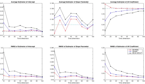
Figure 1: Upper panel: The estimators of the intercept (left), slope (middle) and autoregress-ive parameter (right panel), averaged across the 500 replications, are plotted for N = 30 and T =
{10,20,30,40,50,60,80,100}. The dashed blue lines indicate the true values (used to simulate the data). The red, blue, and black solid lines correspond to the EM-REML, Swamy, and Mean Group estimator, re-spectively. The distances between those lines and the one corresponding to the true value measure the bias of the estimators. Lower panel: the root mean square errors (RMSE) of the estimators are reported.
Regarding the slope coefficient associated to xit, the bias of the EM-REML estimator is
equal to −0.0033 when T = 10, which amounts to −3.3 percent of the true value. When
T = 20, the bias reduces to 1.7 percent of the true value till becoming equal to 0.1 percent when T = 100. In some cases, the EM-REML estimator may have a slightly larger bias than the Swamy one but in all cases it has a smaller or at most equal RMSE.
The advantages in term of bias of the EM-REML approach are even more notable when considering the autoregressive coefficient. For instance, when T = 10, the bias of the EM-REML estimator is equal to 0.0408, which is equivalent to 8.16% of the true value. The biases
of Swamy GLS and the MG estimators of the autoregressive coefficient, when T = 10, are
[image:26.612.76.539.93.362.2]appropriate estimator when either N or T are small.
A graphical summary of these results is provided in Figure 1. The upper panels show the average values (across 500 Monte Carlo replications) of the EM-REML, Swamy, and MG estimators of the average effects. The differences between the latter and the corresponding true values measure the bias of the estimates. The RMSE of the estimators are depicted in the lower panels.
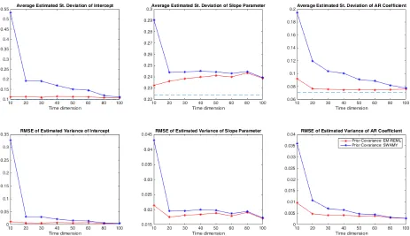
Figure 2: Upper panel: The estimated standard deviation of the intercept (left), slope (middle) and autoregressive parameter (right panel), averaged across the 500 replications, are plotted for N = 30 and T ={10,20,30,40,50,60,80,100}. The dashed blue line indicates the true value (used to simulate the data). The red, and blue lines correspond to the EM-REML, and Swamy estimator, respectively. The distances between those lines and the one corresponding to the true value measure the bias of the estimators. Lower panel: the root mean square errors (RMSE) of the estimated variances are reported.
[image:27.612.75.537.195.464.2]