Color Constancy for Uniform and Non uniform Illuminant Using Image Texture

form and Non-uniform Illuminant Using Image Texture.

IEEE Access.

ISSN 2169-3536 DOI:

https://doi.org/10.1109/ACCESS.2019.2919997

Link to Leeds Beckett Repository record:

http://eprints.leedsbeckett.ac.uk/5936/

Document Version:

Article

The aim of the Leeds Beckett Repository is to provide open access to our research, as required by

funder policies and permitted by publishers and copyright law.

The Leeds Beckett repository holds a wide range of publications, each of which has been

checked for copyright and the relevant embargo period has been applied by the Research Services

team.

We operate on a standard take-down policy.

If you are the author or publisher of an output

and you would like it removed from the repository, please

contact us

and we will investigate on a

case-by-case basis.

Color Constancy for Uniform and Non-Uniform

Illuminant Using Image Texture

MD AKMOL HUSSAIN , AKBAR SHEIKH-AKBARI , AND EDWARD ABBOTT HALPIN

School of Computing, Creative Technology, and Engineering, Leeds Beckett University, Leeds LS6 3QR, U.K.

Corresponding author: Akbar Sheikh-Akbari ([email protected])

ABSTRACT Color constancy is the capability to observe the true color of a scene from its image regardless of the scene’s illuminant. It is a significant part of the digital image processing pipeline and is utilized when the true color of an object is required. Most existing color constancy methods assume a uniform illuminant across the whole scene of the image, which is not always the case. Hence, their performances are influenced by the presence of multiple light sources. This paper presents a color constancy adjustment technique that uses the texture of the image pixels to select pixels with sufficient color variation to be used for image color correction. The proposed technique applies a histogram-based algorithm to determine the appropriate number of segments to efficiently split the image into its key color variation areas. The K-means++algorithm is then used to divide the input image into the pre-determined number of segments. The proposed algorithm identifies pixels with sufficient color variation in each segment using the entropies of the pixels, which represent the segment’s texture. Then, the algorithm calculates the initial color constancy adjustment factors for each segment by applying an existing statistics-based color constancy algorithm on the selected pixels. Finally, the proposed method computes color adjustment factors per pixel within the image by fusing the initial color adjustment factors of all segments, which are regulated by the Euclidian distances of each pixel from the centers of gravity of the segments. The experimental results on benchmark single- and multiple-illuminant image datasets show that the images that are obtained using the proposed algorithm have significantly higher subjective and very competitive objective qualities compared to those that are obtained with the state-of-the-art techniques.

INDEX TERMS Color constancy, multiple-illuminant, image segmentation, texture.

I. INTRODUCTION

The colors of objects within a digital image are determined by the intrinsic properties of the source illuminant, reflective features of the objects’ surface and the sensitivity functions of the imaging device [1]. The color of the illuminant may alter the real colors of the objects within the scene. Hence, for robust color-based systems such as human-computer interac-tion, video analytics, object tracking, color feature extraction and digital photography, the effect of the illuminant should be removed [2], [3]. The retinex system of humans is able to observe the actual color of objects by adjusting its spectral response and distinguishing the color of the source illumi-nant. In contrast to human eyes, digital imaging devices are unable to efficiently filter out the effects of light sources from digital images [4], [5]. Hence, the color of the source light can significantly deteriorate the color of objects in the image. The key purpose of color constancy algorithms is to

The associate editor coordinating the review of this manuscript and approving it for publication was Weiyao Lin.

adjust the color of an image that was taken under an unknown illuminant so that the image looks as if it captured under white illuminant [6], [7].

Color constancy of a digital image can be analyzed using an image formation model. Lambertian reflectance is one the most often used models, which assumes the reflected intensity of the light is independent of the viewing angle. This model ignores the specular reflection. By assuming a Lam-bertian surface, the formation of an imagef =(fR,fG,fB)T becomes a function of three significant factors including the color of the light source I(λ), the sensitivity function of the camera(ρR(λ), ρG(λ), ρB(λ))T, and the reflectance property of the surfaceS(x, λ), whereλ is the light wave-length and x is the spatial coordinate of the object. The formation can then be expressed as follows [8]:

fc(x)=m(x)

Z

w

I(λ)ρc(λ)S(x, λ)dλ (1) wherem(x) refers to the Lambertian shading.

72964

2169-35362019 IEEE. Translations and content mining are permitted for academic research only.

This assumes that the scene is illuminated by a single light source and the perceived color of light sourceedepends on theρ (λ)andI(λ):

e= 



eR eG eB



= ∫

w

I(λ) ρ (λ)dλ (2)

Since camera sensitivity function and the color of the light source are unknown, the color constancy becomes an under-constrained problem that requires additional assump-tions to solve it.

A considerable number of color adjustment methods have been proposed over the past years, where most of them assume that the scene is lit by just one uniform light source [9]–[30]. These algorithms can be classed into four key groups: statistical-, gamut-, physics- and learning-based methods.

Statistical-based color constancy methods use the statis-tical color information of the image to filter out the effect of illuminant color from the image. The Gray World color constancy method [9] is an example of a statistical-based method which is based on the assumption that the average reflectance of the RGB components of a digital image are equal and representative of the gray level. The Gray World algorithm is considered one of the best-performing methods for images that have sufficient color variation [10]. How-ever, its resulting image becomes biased toward the color of the large uniform color patch within the image [11]. Max-RGB, which is also known as the White Patch method, is another statistical-based method, which assumes maximum values of the three image color components represent perfect reflectance [12]. Lam in [13] has taken into account the fact that the human visual system is more delicate to green than red and blue colors. He proposed an algorithm that leaves the green color component of the image unchanged and adjusts the red and blue color components using the Max-RGB method. However, the data dependency of these techniques on the brightest pixels of the image often leads to erroneous results, particularly for images with lower inten-sity [14]. Finlayson and Trezzi [15] proposed a method, which is called Shades of Gray, that overcomes the data reliance of the above two named methods. The authors pro-posed a method that uses the Minkowskip-norm to perform color constancy adjustment. This method generates superior results and significantly reduces the data reliance of the technique. However, in some cases, it generates erroneous and over-saturated images. Several refinement techniques have been proposed in [16]–[18] for alleviating the uniform color areas of the image and improving the result of the aforementioned statistics-based methods. Van de Weijeret al. in [19] have shown that pixels within the edge areas of the image carry important color information and can be used for color constancy adjustment. They proposed a color constancy method that uses the edge pixel information and reported significant results. In [20], an extension of the Gray Edge method, which is named the Weighted Gray Edge method,

was presented. This method incorporates a general weighting scheme of the Gray Edge method by utilizing various edges within the image to perform color constancy adjustment.

Gamut mapping [21] is one of the most remarkable meth-ods. It is based on the principle that for a given light source, in a real-world scene, only a few number of its colors are observable. Various gamut mapping algorithms have been reported in [22]–[24].

Physics-based approaches are more elaborate in their operation, as the light source estimation is driven by the interaction between the source light and the objects’ physical features. They assume that a plane in RGB space represents each surface’s pixels. They use the interaction between these surfaces to estimate the light sources. Many physics-based color constancy methods have been reported in [25]–[28]. Most color constancy methods, including those that are reviewed above, assume that the scene is uniformly lit by only one illuminant. However, in real-life scenarios, the scene is usually lit unevenly by one or more light sources. Hence, current color constancy algorithms are incapable to fully filter out the effects of the light colors.

Researchers have proposed a range of techniques that meet the needs of color constancy adjustment methods for images that were taken from a scene that was either un-evenly lit or lit by multiple light sources [29]–[51]. These methods can be divided into groups that are based on local light estimation and fusion [29]–[34], pixel-detection-based tech-niques [35]–[37], Convolutional Neural Network (CNN)-based methods [42]–[47] and biologically inspired tech-niques [48]–[51].

A superpixel-based segmentation method was proposed in [32], which uses various sub-sampling techniques to split the image into sub-regions and determine a light-source color estimate for each resulting sub-region. Then, the algo-rithm combines the resulting estimates from the same cat-egory to generate a light color estimate for each pixel. Beigpouret al.[33] used the conditional random field algo-rithm, which considers both spatial distribution of local light estimates and their colors, to generate a per-pixel light source color estimate. The authors formulated a framework as an energy minimization task of the spatial distribution, which combines a few physics-based and statistics-based color con-stancy methods into a single color guesstimate for multiple illuminant scene. Another multiple-light-source estimation method was proposed in [34], which uses lattices of vari-ous scales of the image to calculate a per-pixel light color estimate.

In the literature, various color constancy algorithms have also been reported that attempt to perform illumination esti-mation without relying on the presence of particular sets of pixels [38]–[41]. A two-stage color constancy adjustment method for outdoor images was proposed by Leeet al.in [41]. Their algorithm casts the shadow and sunlight as two illumi-nants. In the first step, the algorithm determines an estimate for the sunlight and its reflectance in the whole image using an existing technique that assume the scene is lit by only one light source. In the second step, their algorithm estimates the secondary illuminant, which corresponds to shaded regions of the image, and applies a pixel-based color correction to the shaded regions of the image by calculating the RGB adjustment ratio without estimating the color of shade. Thus, the authors have proposed a way of adopting diverse color constancy approaches for primary and secondary illuminant estimation. They have demonstrated through experiment that their technique generates significantly more accurate results in terms of angular errors on outdoor images.

Several techniques use a convolutional neural network (CNN)-based color constancy approach for multiple illumi-nants as an alternative to the strong-assumption-based meth-ods [42]–[47]. Biancoet al.[42] use a CNN that comprises of one convolutional layer, one fully connected layer, and three output nodes. This method samples the input image into non-overlapping patches and applies the histogram stretching method to neutralize the contrast of the image. The patch scores, which are attained by mining activation values of the last hidden layer, are merged to guess the color of source light. Barron [43] observed that weighting the color components of the image causes a translation in the log-chromaticity histogram of the image, which enables the use of tools such as CNN and structure prediction. Joze and Drew [44] iden-tifies a neighboring surface from the training data by using both inadequately color-constant RGB values and texture features. The authors then integrate them as an illuminant estimation for the whole image. Aytekinet al.[47] proposed another CNN-based color constancy technique that estimates the chromaticity of the light by pooling local patches from an image pyramid. Their algorithm creates the image pyramid, which consists of a few scales of the input image, and extracts local patches from all resolutions. Then, algorithm trains a CNN to estimate the illuminant from the extracted image patches. To eliminate the effect of limited content in small patches, it uses two additional training features, namely, the mean and the median of the local patches, for illuminant estimation.

Various algorithms that endeavor to mimic the mecha-nism of the Human Visual System (HVS) using a compu-tational model for color constancy have been presented in the literature [48]–[51]. Gaoet al.[48] reported a method that is based on the response of Double Opponent (DO) cells to the incident distribution of the color. They apply a max- or sum-pooling mechanism in long-, medium- and short-wavelength color space to estimate the illuminant color. A biologically inspired computational model was proposed

in [50], which depend mainly on center-surround calcula-tions of local contrast to preserve the object color. Their model mimics the coordination between the variable size of the Receptive Field (RF) and its surrounding local contrast by weighting contributions of two overlapping asymmetric Gaussian kernels. Then, the authors estimated the illuminant by modeling higher visual cortical areas according to the local contrasts. A color constancy method that automatically detects the human eyes and extracts the color of the sclera, was proposed by Maleset al.in [51]. The proposed algorithm assumes that the sclera color contains sufficient accurate information to be used to estimate the scene light color and, hence, reliably color-balance the face image. They reported superior performance compared to other techniques. Never-theless, the use of this technique is restricted to images that contain at least one reliable human eye.

Although the aforementioned color constancy methods generate reasonably accurate results, to authors’ knowledge, the application of image texture for color constancy adjust-ment of images of scenes illuminated by multiple light sources has not been reported in the literature. With advances in multimedia technologies, there is increased demand for more reliable, accurate and less computation hungry mul-tiple illuminant color constancy techniques. This paper presents Color Constancy Adjustment using the Texture of the Image (CCATI) for single and multiple illuminants. The proposed technique uses a histogram-based algorithm to determine sufficient number of segments for the input image. The proposed algorithm applies an automatic segmentation method that uses the K-means++_{method to divide the input}

FIGURE 1. An illustrative block diagram of the proposed technique.

II. PROPSOED COLOR CONSTANCY ADJUSTMENT USING IMAGE TEXTURE

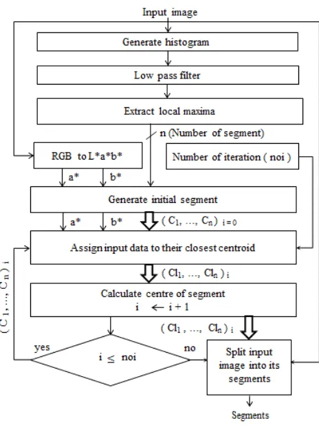
Fig. 1 shows an illustrative block diagram of the proposed technique. In this paper, the K-means++algorithm along with a histogram-based method are used to divide the input image into a number of segments. Our investigation shows that entropy analysis of each image segment provides adequate information about the color variations of the pixels. This information is then used to select pixels with sufficient color variation within each segment. The proposed method deter-mines initial color constancy adjustment factors for each seg-ment using its selected pixels. The proposed method assumes each image segment represents a dominant light source. The proposed method then calculates per pixel, color constancy adjustment factors by combining the resulting initial color constancy adjustment factors of different segments adjusted by the Euclidian distances of the pixel from the centroids of the segments. This enables the algorithm to balance the effect of different light sources represented by different segments on each pixel, globally improving overall color constancy of the image. The proposed color constancy adjustment method includes three parts: automatic image segmentation using the K-means++ algorithm, calculation of the initial color con-stancy weighting factors for each segment and computation of the color constancy adjustment weighting factor for each pixel by fusing the color constancy weighting factors of all segments. These three parts are detailed in the following sub-sections.

A. IMAGE SEGMENTATION USING THE K-MEANS++

ALGORITHM

A block diagram of the proposed automatic image segmentation method, which uses the K-means++clustering algorithm [52], is shown in Fig. 2. According to Fig. 2, the algorithm takes an RGB color image and transforms it into a gray scale image. The algorithm uses a histogram-based method to calculate the number of segments demonstrat-ing color diversity areas within image. Hence, it splits the resulting gray scale image data into 256 bins of a histogram. Then, the resulting histogram is smoothed six times using the

FIGURE 2. Block diagram of the proposed image segmentation algorithm.

following Gaussian low-pass filter:

[0.25 0.5 0.25]

image datasets. The calculated number of segments, which is denoted as n, is shown as n in Fig. 2. Various image segmentation algorithms can be used to split the input image intonsegments. However, in this research, the K-means++ clustering algorithm, which is simple and effective in divid-ing the color image into a predefined number of segments according to the variation of the color data, is used. Hence, the input RGB image is converted to the L∗a∗b∗ format, where the lightness and the color components of the image are denoted by L∗, a∗and b∗, respectively. The a∗and b∗color components and the calculated number of the segmentsnare fed to the K-means++clustering technique.

The K-means++method splits the input image pixels inton segments according to their color variations. The K-means++ segmentation method’s steps are as follows:

i. Randomly select the initialncentroids of the segments from the a* and b* the input image color component, which are named as(c1. . .cn)i=0, and setito zero (i denotes the current iteration).

ii. Segment the a* and b* image color components’ coeffi-cients intonsegments based on their minimum Euclid-ian distances to the currentncentroids, to generaten new segments, which are denoted as(cl1. . .cln)i. iii. Compute the mean value of each resulting segment’s

coefficients to determine thennew centroids, denoted as(c1. . .cn)iin Fig. 2 and increaseiby one.

iv. Check if i is larger than the predefined number of iterations, named as noi in Fig. 2. Ifi is larger than noi, the formerly calculated segments, denoted as

(cl1. . .cln)i, are the final segments and the segmen-tation procedure is complete. Change their name to cl1. . .cln, as shown in Fig. 2, otherwise, back to step ii.

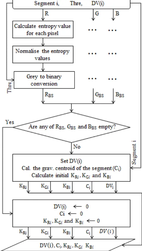
B. TEXTURE EXTRACTION AND CALCULATION OF THE INITIAL CONSTANCY WEIGHTING FACTORS

A block diagram of the proposed texture extraction, segment selection and segment initial color constancy weighting factors computation methods is illustrated in Fig. 3. Each resulting segment from Section 2.1 is processed indepen-dently as follows:

i. Calculate the entropy value for each pixel’s color components of the segment using 9×9 neighboring values [53] (the entropy value is a statistical measure of the randomness and is used to characterize the texture of the segment).

ii. Normalize and map the resulting entropy values to [0, 1].

iii. Convert each resulting normalized color component segment texture map to binary using two empirical threshold values as detailed in the experimental section. iv. If all of the resulting binary color component maps are non-zero, calculate its gravitational center and set the segment’s relevant bit in the decision vector (DV), a vector indicating which segments have been selected that was initialized to zero.

FIGURE 3. Block diagram of the proposed texture extraction, segment selection and segment initial color constancy weighting factor calculation methods.

v. Determine the segment’s initial color constancy weighting factors using the input RGB image pixel values, which are identified by the resulting non-zero binary segment’s pixels. The weighting factors for the red, green and blue color components are denoted as KRi, KGi and KBi, respectively, in the block dia-gram, where irepresents the segment number. Finally, the Gray World theorem is used to compute the weight-ing factors, as shown in equation (3):

KCi=SSPmean

P

SSPC

N (3)

where KCi is the initial weighting factor for component C∈ {R,G,B}; SSPmean is the average value of the seg-ment’s selected pixel values, which are identified by the non-zero binary segment’s pixel values;P

FIGURE 4. Block diagram of the proposed color constancy weighting factor (CCWF) calculation for each pixel by fusing the initial CCWFs of the selected segments.

of component C’s segment’s selected pixel values; and N is the total number of non-zero binary pixels of the binary segment.

In this research, the Gray World color correction algorithm, which is one of the more effective and yet less computation-ally expensive techniques compared to other color constancy algorithms [4], [10], [11], [19], [20], is used for simplicity to compute the initial color constancy weighting factors for segments. However, other statistical color constancy methods can be used.

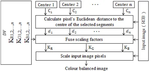
C. CALCULATING THE PER-PIXEL COLOR CONSTANCY WEIGHTING FACTORS

Fig. 4 presents a block diagram of the proposed color constancy adjustment weighting factor calculation method for each pixel. According to Fig. 4, the proposed algo-rithm takes the segments’ centers, which are denoted as C10 C₂0 · · ·,C_n , the RGB input image, the Decision Vector (DV), and the calculated initial color correction weighting factors of all the segments and computes per pixel color correction weighting factors by combining the initial color correction weighting factors of all segments, as explained in the following steps:

i. Calculate the Euclidian distances of the pixel from the centers of all segments, which are denoted as d1, d2,. . . dnin the block diagram, using equation (4):

di =

q

xCi−xp

2

+ yCi −yp

2

(4)

where xCi andyCi are the x andy positions, respectively, of the center of segmenti;xp andyprepresent thex andy positions, respectively, of the pixel in the image; anddiis the Euclidian distance of the pixel from the center of segmenti.

ii. The color constancy adjustment weighting factors for the red, green and blue color component of the pixel, which are denoted as KR, KGand KB, respectively, are calculated by fusing the regulated initial color constan-cies of the segments using equation (5):

Kl =

d1 d1+d2+ · · · +dn

×Kl1+

d2 d1+d2+ · · · +dn

×Kl2+ · · · +

dn

d1+d2+ · · · +dn

×Kln (5)

where Kl is the weighing factor for component l of the pixel;l ∈ {R,G,B}; d1,d2, · · ·,dn represent the Euclid-ian distances of the pixel from the centers of segments 1 ton, respectively, which are denoted as C10 C₂0 · · · ,C_n in the block diagram; and K_l0

1 Kl

0

2

· · ·,Kln are the initial color constancy weighting factors of color componentl of segments 1 ton,respectively.

iii. Scale the R, G and B color components of the input pixel by the resulting color constancy weighting factors using the Von-Kries diagonal model [54], as shown in equation (6):





p_out_R p_out_G p_out_B



= 



KR 0 0

0 KG 0

0 0 KB

    pR pG pB   (6)

wherep_out_R,p_out_Gandp_out_Bare the color components of the color-balanced pixel; KR, KGand KBare the calculated weighting factors for the input pixel; andpR,pGandpBare the input pixel’s color component values.

III. EXPERIMENTAL RESULTS AND EVALUATION METHODS

The performance of the proposed color correction method for images of scenes, which are lit by a various illumi-nant is assessed and compared with those of the state-of-the-art techniques using images from four benchmark image datasets. The remainder of this section is organized as follows: the datasets are introduced in sub-section 3.1; sub-section 3.2 explains the assessment criteria; the influ-ence of various factors on the performance of the proposed algorithm is discussed in sub-section 3.3; and sub-section 3.4 details the experimental results.

A. IMAGE DATASETS

B. MULTIPLE-ILLUMINANT DATASETS

1. The Multiple Light Sources dataset (MLS) [32] con-sists of 9 outdoor images of different sizes, which were captured under two distinct lighting conditions, and 58 indoor images, which were shot under various lighting conditions. The ground truth of the images are also generated using different methods, e.g. by placing several gray balls in the scene and manually correcting the image.

2. The MIMO dataset [33] consists of 58 laboratory and 20 real-world images. The laboratory images were shot under controlled illumination conditions.

C. SINGLE-ILLUMINANT DATASETS

4. The Gehler and Shi image dataset [56] consist of 568 images covering a wide range of indoor and outdoor scenes’ images, which were captured under various lighting conditions. A Macbeth color checker chart was located in a known place of each scene, which its image is used to assess the lighting condition of the scene. One hundred images from this dataset are used for subjective evaluation of the proposed color correction method.

D. ASSESSMENT CRITERIA

To evaluate the color constancy of images, both objective and subjective measures are widely used in the litera-ture [1], [33], [40], [57], [58]. Angular error, which is an objective measure, is often used to assess the color con-stancy of an image when the ground truth of the image is available. In this case, the angular distance between the color-corrected image and its respective ground truth, which is also known as the recovery angular error [59], is determined using equation (7):

d_θ(recovery)= cos−1( e.eˆ

kekˆe

) (7)

whered_θ represents the angular error,e.eˆ indicates the dot product of the ground-truth and the color-corrected image vectors, respectively, andk.kdenotes the Euclidian norm of the specified vector.

Angular error is the most frequently used measure in assessing the performance of color correction techniques, where the average of the mean or median angular errors of various techniques on a large set of color-balanced images is calculated and used for comparison. The images of an algorithm that has the lowest average of the mean or median angular errors have the highest color constancy.

Recently, Finlaysonet al.[60] have criticized the applica-tion of the (recovery) angular error measure based on the argument that it produces different results for identical scenes viewed under different color light sources. They proposed an improved version of the recovery angular error measure, called reproduction angular error, which is defined as the angle between the image RGB of a white surface when the actual and estimated illuminations are ‘divided out’. The reproduction angular error metric can be calculated using equation (8):

d_θ(reproduction)= cos−1 (e/ˆe)

e/ˆe

.w

!

(8)

wherew= e√/eˆ

3 is the true color of the white reference. Both recovery and reproduction angular error have been used to assess the objective quality of the color corrected image by computing the average of the mean or median reproduction angular errors of different methods on a large set of color-corrected images and using them for comparison. The images of the method that have the lowest average of the

mean or median reproduction angular errors have the highest color constancy.

Although angular error often provides very similar results to human perception, contradictory results have also been reported by researchers in [61], [62]. Since human eyes are the ultimate critic of the color constancy of images, subjective evaluation is considered the most reliable assessment method, regardless of its difficulty in terms of time consumption and required resources. Mean opinion score (MOS) is a subjective measure that is widely used to compare the visual quality of color-balanced images [63], [64]. In this method, a set of images that contain various color variations, objects, and backgrounds and are captured under various light sources are selected and color-balanced by various color constancy adjustment techniques. The resulting images are shown to observers who score the images based on their color con-stancy. For comparison, the MOS for each algorithm is gen-erated by considering the average scores for the images of a dataset.

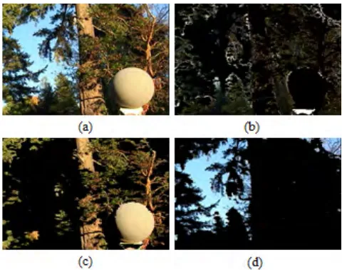
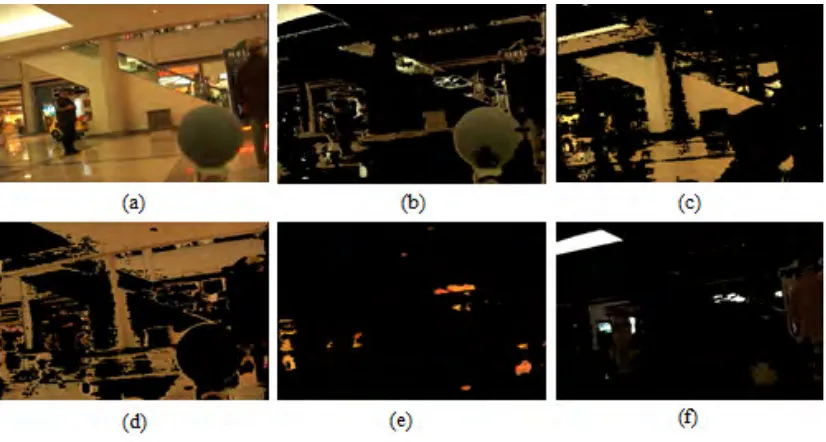
According to Fig. 5, the proposed algorithm divided the input image into three segments, where the pixels within each segment are of similar color and the three segments mainly cover leaves, a tree log, and the ball and the blue sky, respectively.

FIGURE 5. Sample outdoor image from the gray ball dataset and its resulting segments that were obtained using the proposed segmentation algorithm: (a) original image and (b-d) the resulting three segments.

FIGURE 6. Sample indoor image from the gray ball dataset and its resulting segments that were obtained using the proposed segmentation algorithm: (a) original image and (b-f) the resulting five segments.

color correction method. The impact of number of segments on the performance of the proposed color constancy tech-nique will be further investigated in the experimental results section.

E. THRESHOLD SELECTION AND DEMONSTRATION In the proposed algorithm, as explained in Section 2.2, two threshold values are used to extract pixels with sufficient color variation to be used to calculate the initial color con-stancy weighting factors for the segment (these thresholds are applied on the normalized gray entropy pixel values of each segment). This operation also excludes pixels of the uniform-color areas from being used for image color constancy adjustment. In general, the existence of a large uniform-color area causes the color-corrected image to be biased to the color of the large uniform area. The range of the threshold values lies between 0 and 1. To empirically deter-mine lower and upper threshold values, which clearly define areas with sufficient color variation, an extensive empirical investigation on a wide range of images of different datasets was conducted. Initial results showed pixels with normalized entropy value less than 0.05 and above 0.95 mainly repre-sent uniform color areas and areas with significant edges, which do not contain adequate color variation. Hence the initial lower and upper threshold values were initialized to 0.05 and 0.95 prior to empirically determine their values precisely.

The following steps were applied to many sample images from the four abovementioned image datasets to empirically determine the two required threshold values, which are named as the upper and lower threshold values and denoted as Tuand Tl, respectively:

i. Assign 0.05 and 0.95 to Tl and Tu, respectively.

ii. Apply the thresholds to the texture of a segment that contains uniform color areas, e.g., blue sky, and set the unselected pixels of the segment to zero.

iii. Visually inspect the resulting segment.

iv. If the uniform-color area of the segment has almost disappeared, go to step vi.

v. Set Tl= Tl+0.05 and Tu= Tu−0.05 and go to step ii.

vi. The current threshold values are the empirical threshold values for this image.

Then, the average of the resulting threshold values for the selected images from the four datasets were calculated and used as the general empirical values for the proposed method, which are 0.3 and 0.7 for Tl and Tu, respectively.

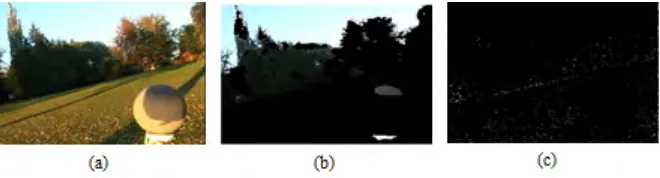
To give a visual sense of the performance of the algorithm, one outdoor image that contains uniform blue sky and one indoor image that contains a uniform-color area were seg-mented using the proposed algorithm. The entropy values of the segments that contain uniform areas were calculated and the general empirical threshold values were applied. The orig-inal images, their uniform-color segments and the resulting selected pixels of the segments are shown in Fig. 7 and Fig. 8. According to Fig. 7c and Fig. 8c, the pixels with adequate color variation are selected by the proposed technique and the uniform-color areas are excluded from contributing to the color constancy correction of the images.

F. EXPERIMENTAL RESULTS

FIGURE 7. Sample outdoor image from the gray ball dataset: (a) original image, (b) a segment that contains a uniform-color area, and (c) selected pixels for color constancy adjustment within the segment that represents the non-uniform-color area.

FIGURE 8. Sample indoor image from the gray ball dataset: (a) original image, (b) a segment that contains the uniform-color area, and (c) selected pixels for color constancy adjustment within the segment that represents the non-uniform-color area.

objective evaluation on a wide range of images of scenes that are lit by either a single or multiple light source.

G. SUBJECTIVE RESULTS

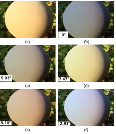
To assess and compare the subjective performance of the proposed CCATI algorithm, five sample images from the four image datasets that contain images that were captured under single and multiple light sources in outdoor, indoor, natural and laboratory settings are color-corrected using the proposed CCATI and the state-of-the-art color correction methods. The results are shown in Fig. 9-14. Fig. 9 illustrates a sample image from the Gray Ball dataset, the ground truth of the image, and color-corrected images that were generated using Gray Edge-2, Weighted Gray Edge, Double Opponency and the proposed CCATI method. According to Fig. 9, the pro-posed method’s image exhibits the highest color constancy, whereas the Weighted Gray Edge, Gray Edge-2 and Dou-ble Opponency images, in order, have visually lower color corrections, which is inconsistent with their angular errors, which are indicated on the images. To obtain better insight into the achieved color constancy, the gray ball areas of the images that are obtained using the various techniques, which correspond to the area that is highlighted by the red window on the original input image, are shown in Fig. 10. According to Fig. 10a, which shows the gray ball part of the input image, the ball color exhibits a strong yellow color cast compared to its ground truth, as shown in Fig. 10b, which illustrates the true gray color of the ball. The Gray Edge-2 method’s image, which is shown in Fig. 10c, exhibits a light brown color cast compared to the ground truth. The Weighted Gray Edge method’s image is illustrated in Fig. 10d. This image

FIGURE 9. Sample image from the gray ball dataset, its ground truth and its color-balanced images: (a) original, (b) ground-truth, (c) Gray Edge-2, (d) Weighted Gray Edge, (e) Double Opponency and (f) the proposed CCATI method’s images.

FIGURE 10. Highlighted area of the sample image from the gray ball dataset, its ground truth and its color-balanced images: (a) original image, (b) ground truth, (c) Gray Edge-2, (d) Weighted Gray Edge, (e) Double Opponency and (f) the proposed CCATI method’s images.

exhibits a high level of orange color cast. Finally, Fig. 10f, which shows the proposed method’s image, seems to have the weakest color cast compare to the other methods’ images and is the closest to the ground-truth image. Therefore, it is con-cluded that the proposed CCATI technique’s images exhibit the uppermost color corrections compared to the other above-mentioned algorithms.

Fig. 11a and 11b show a sample image from the Gray Ball dataset, which seems to have a yellow color cast, and its ground truth, respectively. A large part of this image is the blue sky, which could degrade the performance of the statistical-based color constancy algorithms. According to Fig. 11c, which shows the Max-RGB method’s image, the color cast of the gray ball image, the color cast of the gray ball is very similar to that of the input image. This implies that the Max-RGB algorithm was unable to fully adjust the color of the image. The Shades of Gray algorithm’s image, which is shown in Fig. 11d, exhibits significantly weaker color cast compared to the original image, mostly around the gray ball area of the image, whereas the back-ground of image shows higher yellow color cast than the input image. The Gray Edge-1 technique’s image, which is shown in Fig. 11e, exhibits a similar color casts to that of the Max-RGB method’s image. Although it shows slightly higher color constancy than that of Max-RGB, the gray ball area of its image does not have the pure gray color of the ground-truth image. Fig. 11f shows the Gray Edge-2 method’s image.

FIGURE 11. Sample image from the gray ball dataset, its ground truth and its color-balanced images: (a) original image, (b) ground truth,

(c) Max-RGB, (d) Shades of Gray, (e) Gray Edge-1, (f) Gray Edge-2, (g) Weighted Gray Edge, and (h) Proposed CCATI method’s images.

This image demonstrates superior color constancy, and in particular, the area within the gray ball of this image appears to have a reduced level of yellow tint. Nonetheless, the shore and the tree branches still show some levels of color cast. The Weighted Gray Edge methods’ image, which is shown in Fig. 11g, exhibits a strong yellow color cast; the gray ball, the tree branch and the shore areas of the image seem to have an extremely strong yellow color cast. The proposed CCATI technique’s image is shown in Fig. 11h. This image exhibits the uppermost color correction compared to all the other techniques’ images. The color cast from the tree branches, the shore and the gray ball areas of the image is almost removed and the image is closest in color to the ground-truth image.

FIGURE 12. Sample image from the MIMO (real-image group) dataset, its ground truth and its color-balanced images: (a) original image, (b) ground truth, (c) Gray Edge-2, (d) Weighted Gray Edge, (e) Gray Pixel and (f) the proposed CCATI method’s images.

The Gray Edge-2 algorithm’s image, which is shown in Fig. 12c, does not show a noticeable improvement over the original image. The Weighted Gray Edge’s image, which is shown in Fig. 12d, exhibits an extremely strong blueish color cast. The Gray Pixel method’s image is shown in Fig. 12e. It exhibits significant color correction compared to the Gray Edge-2 and Weighted Grey Edge images, but it still exhibits noticeable differences from the ground-truth image. Fig. 12f shows the proposed CCATI algorithm’s image. This image

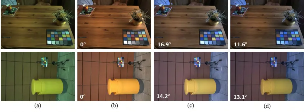
shows uppermost color constancy amongst all the techniques’ images, despite its slight yellow color cast. Moreover, the pro-posed method exhibits the lowest angular error compared to the other techniques’ images. Fig. 13 shows two images and their ground truths from the Gehler and Shi dataset and their respected color-corrected images that were generated using Biancoet al.’s local-to-global regressor and the pro-posed CCATI algorithm. The angular error of each image has been calculated and is shown in the lower-left side of each image. According to Fig. 13a, the original images have various levels of green color cast. According to Fig. 13c and Fig. 13d, which illustrate the Biancoet al.and the proposed algorithm’s images, both methods’ images have a low level of blue color cast. However, the proposed method’s images show much higher color constancy compared to Bianco et al.’s images. By comparing the angular errors of these images, it is concluded that the subjective image quality is in agreement with the objective measures.

Fig. 14 shows an image from the Multiple-Illuminant Light Source dataset, its ground truth and its color-corrected images that were generated using Gray Edge-1, Weighted Gray Edge, Gray Pixel and the proposed CCATI method. According to Fig. 14a, the original image shows a colorful doll that has been placed in front of a multi-colored bag and illuminated by multiple artificial light sources. The luminance of the image background is lower than that of its foreground and parts of the image suffer from red or orange color casts. The Gray Edge-1 technique’s image is shown in Fig. 14c. This image exhibits a noticeable reduction of the color cast on its lower-left side; however, the color cast of the image on its lower-right side is evident. Fig. 14d shows the Weighted Gray Edge method’s image. This image shows superior color constancy than the Gray Edge-1 method’s image; however, it still shows an obvious color cast on its right-hand side. The Gray Pixel technique’s image is shown in Fig. 14e. This image appears to have much weaker color cast than

FIGURE 14. Sample image from the multiple-illuminant light source image dataset, its ground truth and its color-balanced images: (a) original image, (b) ground truth, (c) Gray Edge-1, (d) Weighted Gray Edge, (e) Gray Pixel, and (f) the proposed CCATI method’s images.

previously explained techniques’ images; however, a slight orange color cast on the left side of the image on the carpet and an extreme purple illuminant on the lower-right side of the image are still obvious. The proposed algorithm’s image is illustrated in Fig. 14f. The color of the lower-left side of the image seems as if it has been illuminated by a white light. Comparing this image with other techniques’ images and the ground truth, it is obvious that the proposed method’s image has the closest color constancy to the ground-truth image, despite a slight color cast on the lower-right side of the image. According to the calculated angular errors, which are shown on the images, the proposed image has the lowest angular error, which implies that it has the highest objective quality.

To generate the Mean Opinion Scores (MOSs), 13, 78, 200 and 100 images from the MLS, MIMO, Gray Ball and Gehler and Shi image datasets, respectively, were ran-domly selected and color-balanced using Weighted Gray Edge (WGE), Gray Pixel, Double Opponency, Convolutional Neural Network

(CNN) and the proposed CCATI techniques. The color-corrected images were shown to 10 viewers, who scored the images on a scale from 1 to 5, where score 5 corresponds to excellent and 1 to unacceptable color constancy of the image. The average of the resulting scores for the images of each dataset and color constancy technique were computed and tabulated in Table 1.

According to Table 1, the proposed method’s images have the highest MOSs, which implies that the proposed method’s

TABLE 1.Mean opinion scores (MOSs) of the propsoed CCATI and weighted gray edge (WGE), gray pixel, double opponency, and convolutional neural network (CNN) algorithms.

images have the highest subject color constancy amongst the considered techniques’ images.

H. OBJECTIVE EVALUATION

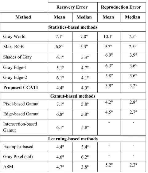
In this section, the performance of the proposed Color Con-stancy Adjustment using the Texture of Image (CCATI) method is objectively compared with those of the state-of-the-art techniques using angular error criteria on images from the four aforementioned datasets. In the first part of the experiment, the images of the Gray Ball dataset were color-balanced using the proposed CCATI, the Gray World, the Max-RGB, the Shades of Gray, the 1st- and 2nd-Order Gray Edge, the Pixel-based Gamut Mapping, the Edge-based Gamut Mapping, the Intersection-based Gamut, the Exem-plar, the Gray Pixel and the Adaptive Surround Modula-tion (ASM) color constancy methods. The average mean and median of both recovery and reproduction angular errors of the color-balanced images are tabulated in Table 2. Accord-ing to Table 2, the proposed CCATI technique’s images have the lowest average mean and median recovery and reproduction angular errors amongst all the statistics- and gamut-based color constancy methods, which implies that the proposed technique’s images have the uppermost objective color constancies compare to the images of the statistics- and gamut-based techniques. With respect to the learning-based

TABLE 3. Average mean and median angular errors of color constancy methods’ images from the mimo dataset.

methods, the proposed technique’s average mean angular error equals 4.4◦, which is equal to the lowest angular error of the learning-based methods. 4.0◦. The proposed algo-rithm’s mean reproduction angular error is 3.9◦, which is the lowest amongst all techniques and However, the proposed algorithm’s average median angular error equals 4.1◦, which is slightly higher than that of the best-performing learning-based method, namely, the exemplar-learning-based method, which is the median reproduction angular error is 3.2◦, which is lower than those of the statistics and gamut-based methods. This demonstrates that the proposed method’s images have very competitive objective results compared to those of the learning-based methods.

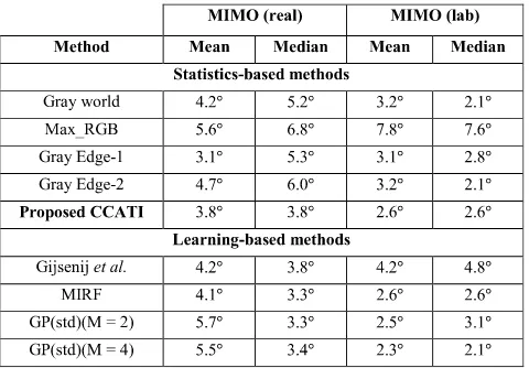
In the second part of the experiment, the images of the MIMO dataset were color balanced using the proposed CCATI, the Gray World, Max-RGB and Shades of Gray, 1st- and 2nd Order Gray Edge, Gisenji et al., MIRF and Gray Pixel (GP) color constancy methods. The average mean and median angular errors of the color-corrected real and laboratory images that were obtained via different the var-ious techniques were determined and tabulated in Table 3. From Table 3 it can be seen that the proposed technique’s MIMO (real) images have the lowest average median and the second-lowest mean angular errors between the images of the statistics-based techniques. Moreover, the proposed method’s MIMO laboratory images exhibit the lowest mean and the second-lowest median angular errors. Hence, it is concluded that the proposed method’s images have almost the

uppermost objective color constancy compared to those of the statistical-based methods. Compared to those of the learning-based methods, the proposed technique’s images have very competitive objective qualities.

Table 4 presents the average median angular errors of the proposed CCATI, the Max-RGB, Gray World, Gray Edge-1, Gray Edge-2 and Gisenjiet al.methods on 9 outdoor images from the Multiple Light Source dataset. According to this table, the proposed techniques’ images have the low-est median angular errors amongst all the techniques. From the objective results that are presented in Tables 2-4, it is concluded that the proposed CCATI method’s images exhibit almost the uppermost objective color constancy compared to the images of the other considered techniques.

TABLE 4. Average median angular errors of the proposed CCATI and other color constancy methods on 9 outdoor images from the multiple light source dataset.

I. PERFORMANCE EVALUATION FOR A FIXED NUMBER OF SEGMENTS VERSUS AUTOMATIC SEGMENTATION

In this section, it will be empirically shown that the appli-cation of the automatic segmentation algorithm significantly improves the performance of the proposed color constancy technique. To do this, the proposed technique, with and without its automatic segmentation method, is applied to the images of the MIMO (real), MIMO (laboratory) and Multiple Light Sources (MLS) (outdoor images) image datasets. The average median angular errors of the resulting images were calculated and are tabulated in Table 5. Results highlight that the proposed method’s images have the lowest average angular error when the proposed technique uses its automatic segmentation algorithm rather than a fixed number of seg-ments.

J. COMPUTATIONAL COMPLEXITY

TABLE 5. Angluar errors of the propsoed method for different numbers of segments.

more computation time than the benchmark Grey World method.

IV. CONCLUSION

In this paper, the Color Constancy Adjustment using the Texture of Image (CCATI) method was presented. The pro-posed technique employs a histogram-based method to effi-ciently calculate the sufficient number of segments for the input image according to the image’s color variation. Then, the algorithm applies a K-means++ method on the input image, which divides the input image into segments. It deter-mines the entropy of the pixels within each segment and uses it to choose pixels with sufficient color variation for calculating the initial color constancy weighting factors for the segment and reduce the effect of large uniform-color areas on the overall performance of the algorithm. Finally, the proposed CCATI method calculates per pixel color cor-rection adjustment factors by regulating the resulting initial color constancy weighting factors of all segments using the Euclidian distances of the pixel from the centers of gravity of all segments. Experimental results were generated using four benchmark image datasets. The results showed the merit of the proposed technique.

REFERENCES

[1] N. Banić and S. Lončarić, ‘‘Color cat: Remembering colors for illumina-tion estimaillumina-tion,’’IEEE Signal Process. Lett., vol. 22, no. 6, pp. 651–655, Jun. 2013.

[2] G. Schaefer, S. Hordley, and G. Finlayson, ‘‘A combined physical and statistical approach to colour constancy,’’ inProc. IEEE Comput. Soc. Conf. Comput. Vis. Pattern Recognit., vol. 1, Jun. 2005, pp. 148–153. [3] T. Jiang, D. Nguyen, and K.-D. Kuhnert, ‘‘Auto white balance using

the coincidence of chromaticity histograms,’’ in Proc. 8th Int. Conf. Signal Image Technol. Internet Based Syst., Naples, Italy, Nov. 2012, pp. 201–208.

[4] A. Gijsenij and T. Gevers, ‘‘Color constancy by local averaging,’’ inProc. 14th Int. Conf. Image Anal. Process. Workshops (ICIAPW), Modena, Italy, Sep. 2007, pp. 171–174.

[5] J. Simão, H. J. A. Schneebeli, and R. F. Vassallo, ‘‘An iterative approach for color constancy,’’ inProc. Joint Conf. Robot., SBR-LARS Robot. Symp. Robocontrol, Sao Carlos, Brazil, Oct. 2014, pp. 130–135.

[6] H. R. V. Joze and M. S. Drew, ‘‘White patch gamut mapping colour constancy,’’ inProc. 19th IEEE Int. Conf. Image Process., Orlando, FL, USA, Sep. 2012, pp. 801–804.

[7] S. J. J. Teng, ‘‘Robust algorithm for computational color constancy,’’ in Proc. Int. Conf. Technol. Appl. Artif. Intell., Hsinchu, Taiwan, Nov. 2014, pp. 1–8.

[8] M. A. Hussain and A. S. Akbari, ‘‘Color constancy adjustment using sub-blocks of the image,’’IEEE Access, vol. 6, pp. 46617–46629, 2018. [9] G. Buchsbaum, ‘‘A spatial processor model for object colour perception,’’

J. Franklin Inst., vol. 310, no. 1, pp. 1–26, Jul. 1980.

[10] S.-C. Tai, T.-W. Liao, Y.-Y. Chang, and C.-P. Yeh, ‘‘Automatic white balance algorithm through the average equalization and threshold,’’ in Proc. 8th Int. Conf. Inf. Sci. Digit. Content Technol., Jun. 2012, pp. 571–576.

[11] A. Gijsenij, T. Gevers, and J. Van de Weijer, ‘‘Computational color con-stancy: Survey and experiments,’’IEEE Trans. Image Process., vol. 20, no. 9, pp. 2475–2489, Sep. 2011.

[12] E. H. Land, ‘‘The retinex theory of color vision,’’Sci. Amer., vol. 237, no. 6, pp. 108–129, Dec. 1977.

[13] E. Y. Lam, ‘‘Combining gray world and retinex theory for automatic white balance in digital photography,’’ inProc. 9th Int. Symp. Consum. Electron., (ISCE), Jun. 2005, pp. 134–139.

[14] N. Banić and S. Lončarić, ‘‘Improving the white patch method by sub-sampling,’’ inProc. IEEE Int. Conf. Image Process. (ICIP), Paris, France, Oct. 2014, pp. 605–609.

[15] G. D. Finlayson and E. Trezzi, ‘‘Shades of gray and colour constancy,’’ in Proc. IST/SID Color Imag. Conf., vol. 1, Jan. 2004, pp. 37–41.

[16] M. A. Hussain, A. Sheikh Akbari, and B. Mallik, ‘‘Colour constancy using sub-blocks of the image,’’ inProc. Int. Conf. Signals Electron. Syst. (ICSES), Krakow, Poland, Sep. 2016, pp. 113–117.

[17] M. A. Hussain, A. Sheikh Akbari, and A. Ghaffari, ‘‘Colour constancy using K-means clustering algorithm,’’ inProc. 9th Int. Conf. Develop. eSyst. Eng. (DeSE), Liverpool, U.K., Aug. 2016, pp. 283–288.

[18] M. A. Hussain and A. S. Akbari, ‘‘Max-RGB based colour constancy using the sub-blocks of the image,’’ inProc. 9th Int. Conf. Develop. eSyst. Eng. (DeSE), Liverpool, U.K., Aug. 2016, pp. 289–294.

[19] J. van de Weijer, T. Gevers, and A. Gijsenij, ‘‘Edge–based color con-stancy,’’ IEEE Trans Image Process., vol. 16, no. 9, pp. 2207–2214, Sep. 2007.

[20] A. Gijsenij, T. Gevers, and J. Van de Weijer, ‘‘Improving color constancy by photometric edge weighting,’’IEEE Trans. Pattern Anal. Mach. Intell., vol. 34, no. 5, pp. 918–929, May 2012.

[21] D. A. Forsyth, ‘‘A novel algorithm for color constancy,’’Int. J. Comput. Vis., vol. 5, no. 1, pp. 5–35, Aug. 1990.

[22] G. D. Finlayson, S. D. Hordley, and I. Tastl, ‘‘Gamut constrained illuminant estimation,’’Int. J. Comput. Vis., vol. 67, no. 1, pp. 93–109, Apr. 2006. [23] G. Finlayson and S. Hordley, ‘‘Improving gamut mapping color

con-stancy,’’IEEE Trans. Image Process., vol. 9, no. 10, pp. 1774–1783, Oct. 2000.

[24] M. Mosny and B. Funt, ‘‘Cubical gamut mapping colour constancy,’’in Proc. Conf. Colour Graph., Imag., Vis., Jan. 2014, pp. 466-470. [25] H.-C. Lee, ‘‘Method for computing the scene-illuminant chromaticity from

specular highlights,’’J. Opt. Soc. Amer. A, Opt. Image Sci., vol. 3, no. 14, pp. 1694–1699, Oct. 1986.

[26] S. Tominaga and B. A. Wandell, ‘‘Standard surface-reflectance model and illuminant estimation,’’J. Opt. Soc. Amer. A, Opt. Image Sci., vol. 6, no. 4, pp. 576–584, Apr. 1989.

[27] Y.-Y. Liao, J.-S. Lin, and S.-C. Tai, ‘‘Color balance algorithm with zone system in color image correction,’’ inProc. 6th Int. Conf. Comput. Sci. Converg. Inf. Technol. (ICCIT), Seogwipo-Si, South Korea, Nov. 2011, pp. 167–172.

[28] S.-M. Woo, S.-H. Lee, J.-S. Yoo, and J.-O. Kim, ‘‘Improving color con-stancy in an ambient light environment using the phong reflection model,’’ IEEE Trans. Image Process., vol. 27, no. 4, pp. 1862–1877, Apr. 2018. [29] M. A. Hussain and A. S. Akbari, ‘‘Color constancy algorithm for

mixed-illuminant scene images,’’IEEE Access, vol. 6, pp. 8964–8976, 2018. [30] C. Riess, E. Eibenberger, and E. Angelopoulou, ‘‘Illuminant color

esti-mation for real-world mixed-illuminant scenes,’’ inProc. IEEE Int. Conf. Comput. Vis. Workshops (ICCV), Nov. 2011, pp. 782–789.

[31] M. Bleier, C. Riess, S. Beigpour, E. Eibenberger, E. Angelopoulou, T. Tröger, and A. Kaup, ‘‘Color constancy and non-uniform illumination: Can existing algorithms work,’’ inProc. IEEE Int. Conf. Comput. Vis. Workshops (ICCV), Nov. 2011, pp. 774–781.

[33] S. Beigpour, C. Riess, J. van de Weijer, and E. Angelopoulou, ‘‘Multi-illuminant estimation with conditional random fields,’’IEEE Trans. Image Process., vol. 23, no. 1, pp. 83–96, Jan. 2014.

[34] L. Mutimbu and A. Robles-Kelly, ‘‘Multiple illuminant color estimation via statistical inference on factor graphs,’’IEEE Trans. Image Process., vol. 25, no. 11, pp. 5383–5396, Nov. 2016.

[35] K.-F. Yang, S.-B. Gao, and Y.-J. Li, ‘‘Efficient illuminant estimation for color constancy using grey pixels,’’ inProc. IEEE Conf. Comput. Vis. Pattern Recognit. (CVPR), Jun. 2015, pp. 2254–2263.

[36] B. Mazin, J. Delon, and Y. Gousseau, ‘‘Estimation of illuminants from projections on the planckian locus,’’IEEE Trans. Image Process., vol. 24, no. 6, pp. 1944–1955, Jun. 2015.

[37] S. Bianco and R. Schettini, ‘‘Adaptive color constancy using faces,’’ IEEE Trans. Pattern Anal. Mach. Intell., vol. 36, no. 8, pp. 1505–1518, Aug. 2014.

[38] N. Elfiky, T. Gevers, A. Gijsenij, and J. Gonzàlez, ‘‘Color constancy using 3D scene geometry derived from a single image,’’IEEE Trans. Image Process., vol. 23, no. 9, pp. 3855–3868, Sep. 2014.

[39] D. Cheng, B. Price, S. Cohen, and M. S. Brown, ‘‘Beyond white: Ground truth colors for color constancy correction,’’ inProc. IEEE Int. Conf. Comput. Vis. (ICCV), Santiago, Chile, Dec. 2013, pp. 298–306. [40] D. Cheng, A. Kamel, B. Price, S. Cohen, and M. S. Brown, ‘‘Two

illu-minant estimation and user correction preference,’’ inProc. IEEE Conf. Comput. Vis. Pattern Recognit. (CVPR), Jun. 2016, pp. 469–477. [41] S.-H. Lee, S.-M. Woo, J.-H. Choi, and J.-O. Kim, ‘‘Two-step

multi-illuminant color constancy for outdoor scenes,’’ inProc. IEEE Int. Conf. Image Process. (ICIP), Beijing, China, Sep. 2017, pp. 710–714. [42] S. Bianco, C. Cusano, and R. Schettini, ‘‘Color constancy using CNNs,’’

inProc. IEEE Conf. Comput. Vis. Pattern Recognit. Workshops (CVPRW), Jun. 2015, pp. 81–89.

[43] J. T. Barron, ‘‘Convolutional color constancy,’’ inProc. IEEE Int. Conf. Comput. Vis. (ICCV), Jun. 2015, pp. 379–387.

[44] H. R. V. Joze and M. S. Drew, ‘‘Exemplar-based color constancy and multiple illumination,’’IEEE Trans. Pattern Anal. Mach. Intell, vol. 36, no. 5, pp. 860–873, May 2014.

[45] D. Fourure, R. Emonet, E. Fromont, D. Muselet, A. Trémeau, and C. Wolf, ‘‘Mixed pooling neural networks for color constancy,’’ inProc. IEEE Int. Conf. Image Process., Phoenix, AZ, USA, Sep. 2016, pp. 3997–4001. [46] S. Bianco, C. Cusano, and R. Schettini, ‘‘Single and multiple illuminant

estimation using convolutional neural networks,’’IEEE Trans. Image Pro-cess., vol. 26, no. 9, pp. 4347–4362, Sep. 2017.

[47] C. Aytekin, J. Nikkanen, and M. Gabbouj, ‘‘Deep multi-resolution color constancy,’’ inProc. IEEE Int. Conf. Image Process. (ICIP), Beijing, China, Sep. 2017, pp. 3735–3739.

[48] S.-B. Gao, K.-F. Yang, C.-Y. Li, and Y.-J. Li, ‘‘Color constancy using double-opponency,’’IEEE Trans. Pattern Anal. Mach. Intell., vol. 37, no. 10, pp. 1973–1985, Oct. 2013.

[49] X.-S. Zhang, S.-B. Gao, R.-X. Li, X.-Y. Du, C.-Y. Li, and Y.-J. Li, ‘‘A reti-nal mechanism inspired color constancy model,’’IEEE Trans. Image Pro-cess., vol. 25, no. 3, pp. 1219–1232, Mar. 2016.

[50] A. Akbarinia and C. A. Parraga, ‘‘Color constancy beyond the classical receptive field,’’IEEE Trans. Pattern Anal. Mach. Intell., vol. 40, no. 9, pp. 2081–2094, Sep. 2018.

[51] M. Males, A. Hedi, and M. Grgic, ‘‘Colour balancing using sclera colour,’’ IET Image Process., vol. 12, no. 3, pp. 416–421, Mar. 2018.

[52] D. Arthur and S. Vassilvitskii, ‘‘K-means++: The advantages of careful seeding,’’ inProc. 18th Annu. ACM-SIAM Symp. Discrete Algorithms, 2007, pp. 1027–1035.

[53] R. C. Gonzalez, R. E. Woods, and S. L. Eddins, ‘‘Representa-tion and descrip‘‘Representa-tion,’’ in Digital Image Processing Using MATLAB. Upper Saddle River, NJ, USA: Prentice-Hall, 2003, ch. 11, pp. 464–4613. [54] J. von Kries, ‘‘Influence of adaptation on the effects produced by luminous stimuli,’’ inSources of Color Science, D. L. MacAdam, Ed. Cambridge, MA, USA: MIT Press, 1970, pp. 109–119.

[55] F. Ciurea and B. Funt, ‘‘A large image database for color constancy research,’’ inProc. 11th Color Imag. Conf. Imag. Sci. Technol., Jan. 2003, pp. 160–164.

[56] P. V. Gehler, C. Rother, A. Blake, T. Minka, and T. Sharp, ‘‘Bayesian color constancy revisited,’’ inProc. IEEE Conf. Comput. Vis. Pattern Recognit. (CVPR), Jun. 2008, pp. 1–8.

[57] S. Wang, Y. Zhang, P. Deng, and F. Zhou, ‘‘Fast automatic white balancing method by color histogram stretching,’’ inProc. 4th Int. Congr. Image Signal Process., Shanghai, China, Oct. 2011, pp. 979–983.

[58] B. Zhang and A. U. Batur, ‘‘A real-time auto white balance algorithm for mobile phone cameras,’’ inProc. IEEE Int. Conf. Consum. Electron. (ICCE), Las Vegas, NV, USA, Jan. 2012, pp. 1–4.

[59] S. D. Hordley and G. D. Finlayson, ‘‘Re-evaluating color constancy algo-rithms,’’ inProc. 17th Int. Conf. Pattern Recognit., vol. 1, Aug. 2004, pp. 76–79.

[60] G. D. Finlayson, R. Zakizadeh, and A. Gijsenij, ‘‘The reproduction angular error for evaluating the performance of illuminant estimation algorithms,’’ IEEE Trans. Pattern Anal. Mach. Intell., vol. 39, no. 7, pp. 1482–1488, Jul. 2017.

[61] L. Shi, W. Xiong, and B. Funt, ‘‘Illumination estimation via thin-plate spline interpolation,’’J. Opt. Soc. Amer. A, Opt. Image Sci., vol. 28, no. 5, pp. 940–948, 2011.

[62] A. Gijsenij, T. Gevers, and M. P. Lucassen, ‘‘Perceptual analysis of distance measures for color constancy algorithms,’’J. Opt. Soc. Amer. A, Opt. Image Sci., vol. 26, no. 10, pp. 2243–2256, 2009.

[63] S. Bianco, L. Celona, P. Napoletano, and R. Schettini, ‘‘On the use of deep learning for blind image quality assessment,’’Signal, Image Video Process., vol. 12, no. 2, pp. 355–362, Feb. 2018.

[64] R. C. Streijl, S. Winkler, and D. S. Hands, ‘‘Mean opinion score (MOS) revisited: Methods and applications, limitations and alternatives,’’ Multi-media Syst., vol. 22, no. 2, pp. 213–227, Mar. 2016.

MD AKMOL HUSSAIN received the B.Eng. degree in electronics and communication from the University of Wolverhampton, in 2011, and the master’s degree (Mainly by Research) from the University of Gloucestershire, in 2014. He is currently pursuing the Ph.D. degree with Leeds Beckett University, U.K. His research interests include computer vision, image processing, and image forensics.

AKBAR SHEIKH-AKBARI received the B.Sc. (Hons.), M.Sc. (Distinction), and Ph.D. degrees in electronic and electrical engineering, 1992, 1995, and 2005, respectively. After completing the Ph.D. degree at the University of Strathclyde in the field of stereo/multi-view video processing, he contin-ued his career in industry, worked on real-time embedded video analytics systems. He is currently a Senior Lecturer with the School of Comput-ing, Creative Technologies & EngineerComput-ing, Leeds Beckett University. His main research interests include signal processing, hyperspectral image processing, source camera identification, image/video forgery, image hashing, biometric identification techniques, assisted living technologies, compressive sensing, camera tracking using retro-reflective materials, standard and non-standard image/video codecs, e.g., H.264 and HEVC, multi-view image/video processing, color constancy techniques, resolution enhancement methods, edge detection in low-SNR environments, and medical image processing.