Enhanced NSGA-II Algorithm for Solving Multiobjective Optimization Problems Using PBX Crossover and POM Mutation.

(1)

Enhanced NSGA-II Algorithm for Solving

Multi-objective Optimization Problems Using PBX

Crossover and POM Mutation.

Ankita Golchha

#

_{, Shahana Gajala Qureshi}

*

#

_{M.Tech (CSE) Scholar, RIT College, Raipur, CSVTU University,}

Bhilai, Chhattisgarh, India

*

_{Asst. Professor, Department of (CSE), RIT College, Raipur, CSVTU University,}

Bhilai, Chhattisgarh, India

Abstract— Non-Dominated Sorting Genetic Algorithm (NSGA-II) is an algorithm given to solve the Multi-Objective Optimization (MOO) problems. NSGA-II is one of the most widely used algorithms for solving MOO problems. The present work proposed as advancement to the existing NSGA-II. It this method, combination of crossover and mutation operators is used other than that in the original NSGA-II, and the results are compared to see if which works better.

Keywords— NSGA-II, Parent-centric Blend Crossover, Power Mutation.

I. INTRODUCTION

The use of technology has increased rapidly over the years and so has increased the usage of software. This makes it important to maintain the quality of the software. Software testing is the most significant analytic quality assurance measure consuming at least 50% of software development cost [3]. The automation process of test data generation is a way that will reduce the time taken up by this task. Genetic Algorithm (GA) is used for this purpose.

A number of multi-objective evolutionary algorithms have been suggested earlier. Non-Dominated Sorting Genetic Algorithm (NSGA-II) is an algorithm given to solve the Multi-Objective Optimization (MOO) problems. It was proposed by Deb et.al in 2002 [4], advancing on the concept given by Goldberg 1989 [1]. NSGA-II is one of the most widely used algorithms for solving MOO problems. Rest of the paper is organized as follows: NSGA-II in second section, Proposed Methodology in third section.

II. NSGA-II

A. NSGA-II

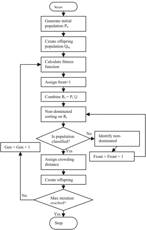
A number of multi-objective evolutionary algorithms have been suggested earlier such as Pareto Archived Evolution Strategy (PAES) & Strength Pareto Evolutionary Algorithm (SPEA), Non-Dominated Sorting GA (NSGA) etc. The Non-dominated Sorting Genetic Algorithm [4] NSGA-II uses a faster sorting procedure, an elitism preserving approach and a parameter less niching operator. The working is given as follows [6]:

Fig. 1 WORKING OF NSGA II Start

Generate initial population P0

Create offspring population Q0e

Calculate fitness function

Assign front=1

Combine Rt = Pt ⋃

Non-dominated sorting on Rt

Identify non-dominated i di id l

Front = Front + 1 Assign crowding

distance

Create offspring Gen = Gen + 1

Stop Is population classified?

Max iteration reached?

Yes No

No

(2)

FIG.2.CREATINGOFFSPRING

B. Selection [7]

In original NSGA II Binary tournament selection (BTS) is used, where tournament is played between two solutions and better is selected and placed in mating pool. Two other solutions are again taken and another slot in mating pool is filled. It is carried in such a way that every solution can be made to participate in exactly 2 tournaments.

C. Crossover [8]

In NSGA II Simulated Binary Crossover (SBX) is used, which works with two parents solutions and create two offspring. The following step-by-step procedure is followed:

Step 1: Choose a random number u ϵ 0,1 ,

Step 2: Calculate using equation 1, Step 3: Compute offspring using equation 2. The mathematical formulation can be given as follows:

β 2u η _{if u 0.5 ;} η

otherwise. (1)

x , 0.5 1 β x , 1 β x , ,

x , 0.5 1 β x , 1 β x , . (2) Here,

u : Random number such that ui ϵ [0, 1],

η : Distribution index (Non-negative real number),

x , & x , : Parent solutions,

x , & x , : Offspring solutions.

D. Mutation [8]

In NSGA II Polynomial mutation is used, which mutates each solution separately, i.e. one parent solution gives one offspring after being mutated. The mathematical formulation can be given as:

y , x , x x δ , (3) Where,

δ 2r 1 if r 0.5,

1 2 1 r , if r 0.5. (4)

Here,

r : Random number such that ui ϵ [0, 1],

η : Distribution index (Non-negative real number),

x , _{: Parent solution,}

x : Upper bound of parent solution,

x : Lower bound of parent solution,

y _{: Offspring solution.}

E. Crowded Tournament Selection [6]

To get an estimation of the density of solutions close to a particular solution i in the population, we take the average of the two solutions on the either side of solution i along each of the objective. This quantity di is the Crowding Distance. The

following algorithm is used to calculate the crowding distance of each point in the set Ƒ .

Assignment procedure: Crowding-sort Ƒ,

Step 1: Call the number of solutions in as Ɩ |Ƒ|. For each i in the set, first assign d 0.

Step 2: For each objective function m 1, 2, . . . , M, sort the set in worse order of f . Find sorted indices vector I sort f , . Step 3: For m 1, . . . , M, assign a large distance to the edge solutions, d d ∞, and for all other solutions j

2 to l 1 , assign:

(5)

III. P

ROPOSED

M

ETHODOLOGY

This section gives an overview of the proposed methodology. In the proposed work we replace the crossover and mutation used in original NSGA-II, Simulated Binary Crossover (SBX) and Polynomial Mutation (PM) are replaced by Parent-Centric Blend Crossover (PBX) [5] and Power Mutation (POM). Also the Binary tournament selection procedure is excluded in a hope to get better result.

A. Parent-Centric Blend Crossover (PBX)

PBX or PBX-α is an extension to BLX-α [3] and is described as follows: Let us assume that X x … x and

Y y … y x , y ϵ a , b ⊂ , i 1 … n are two real-coded variables that have been selected to apply the crossover operator to them. PBX- α generates (randomly) one of these two possible offspring:

Z z … z ) or Z z … z ), (6) Where z is a randomly (uniformly) chosen number from the interval l , u with

l max a , x I ∗α And u min b , x I ∗α (7) And z is chosen from l , u with

l max a , y I And u min b , y I ∗α (8) Where I |x y |.

B. Power Mutation (POM)

In [2] a new mutation operator called Power Mutation (POM) was introduced for real coded genetic algorithms.

The following formula is used to form the mutated solution:

x́ _xx _{s u}s x l , if t_{x , if t} _α (9) Where l and u are lower and upper bounds of the decision variable and α is a uniformly distributed random number between 0 and 1, and s is a random number.

Parent Population

Selection

Crossover

Mutation

(3)

C. Problem Statement

In [9] Schaffer gave two-objective problems:

SCH1 Minimize f x x

Minimize f x x 2 (10)

-A ≤ x ≤ A.

Schaffer’s second function, SCH2,

SCH2

minimize f x

x if x 1, x 2 if 1 3,

4 x if 3 4, x 4 if x 4, minimize f x x 5

5 10

(11)

IV. P

ARAMETER

S

ETUP

F

OR

E

XPERIMENT

In this paper parameter settings are as; Population size = 20, Maximum number of cycles (MCN) = 100. η 20, η 20,

α 0.7, s 0.3.

(X-axis represents f1 & y-axis represents f2.)

TABLE 1

TIME TAKEN IN MILLISECONDS

Problem Combination With BTS Without BTS

SCH1

SBX-PM 145 140

SBX-POM 136 138

PBX-PM 140 143

PBX-POM 133 140

SCH2

SBX-PM 130 174

SBX-POM 128 140

PBX-PM 132 168

PBX-POM 125 150

TABLE 2

GENERATION 100 SCH1 SBX-PM

With BTS Without BTS

F1 F2 F1 F2 2.371634 0.21159 3.975206 3.85E-05 2.298813 0.234078 3.975034 3.91E-05 2.298813 0.234078 3.926204 0.000344 2.242577 0.252482 3.906979 0.000547 2.371634 0.21159 3.881965 0.000884 2.242577 0.252482 3.833179 0.001777 2.242577 0.252482 3.665175 0.007316 2.412973 0.199474 3.492437 0.017212 2.242577 0.252482 3.384913 0.02566 2.371634 0.21159 3.358004 0.028061 2.298813 0.234078 3.317818 0.031867 3.956474 0.000119 3.242758 0.039694 2.412973 0.199474 3.240626 0.039931 2.298813 0.234078 3.234235 0.040643 2.419103 0.197717 3.225016 0.041684 2.412973 0.199474 3.211284 0.043262 2.242577 0.252482 3.182015 0.046734 2.371634 0.21159 3.158029 0.049691 2.371634 0.21159 3.129007 0.053407 2.298813 0.234078 3.099577 0.057331

TABLE 3

G

ENERATION

100 SCH1 SBX-POM

F1 F2 F1 F2 11.68477 2.011575 3.940092 0.000226 11.68477 2.011575 3.620334 0.009464 11.68477 2.011575 3.602233 0.010413 11.68477 2.011575 3.575823 0.011884 11.68477 2.011575 3.572489 0.012077 11.68477 2.011575 3.129007 0.053407 11.68477 2.011575 2.995855 0.07244 11.68477 2.011575 2.794075 0.10788 11.68477 2.011575 2.767892 0.113099 11.68477 2.011575 2.686809 0.130214 11.68477 2.011575 2.655617 0.137191 11.68477 2.011575 2.581277 0.154736 11.68477 2.011575 1.891265 0.390334 11.68477 2.011575 1.834229 0.416881 11.68477 2.011575 1.826128 0.420756 11.68477 2.011575 1.781243 0.442714 11.68477 2.011575 1.740478 0.463391 11.68477 2.011575 1.236766 0.788366 11.68477 2.011575 0.626938 1.459761 11.68477 2.011575 4.023694 3.50E-05

GRAPH1SCH1-SBX-PM

TABLE 8

0

0.2

0.4

0.6

0.8

1

0

1

2

3

4 Optimal

WITH

BTS

WITHOU

T BTS

0

0.2

0.4

0.6

0.8

1

0

1

2

3

4 Optimal

WITH

BTS

(4)

GRAPH 2 SCH1- SBX-POM

GRAPH 3 SCH1- PBX-PM

TABLE 4

GENERATION 100 SCH1 PBX-PM

F1 F2 F1 F2 1.445665 0.636233 3.851107 0.001412 1.269581 0.762554 3.711798 0.005387 1.25942 0.770465 3.64839 0.008086 1.286101 0.749845 3.466731 0.019067 1.445665 0.636233 3.464534 0.019231 1.25942 0.770465 3.422077 0.022534 1.286101 0.749845 3.406209 0.023842 1.861604 0.40398 3.373661 0.02665 1.25942 0.770465 3.129007 0.053407 1.25942 0.770465 2.979971 0.074934 1.269581 0.762554 2.944412 0.080696 1.269581 0.762554 2.942353 0.081038 1.861604 0.40398 2.912155 0.08614 1.25942 0.770465 2.897923 0.088608 1.862868 0.403391 2.891989 0.089649 1.861604 0.40398 2.891989 0.089649 1.286101 0.749845 2.742219 0.11836

1.25942 0.770465 2.726811 0.121588 1.445665 0.636233 2.674732 0.132889

1.25942 0.770465 2.630781 0.142908

GRAPH 4 SCH1- PBX-POM

TABLE 5

G

ENERATION

100 SCH1 PBX-POM

F1 F2 F1 F2 10.21206 1.429535 3.807913 0.002363 10.21206 1.429535 3.789182 0.002853 10.21206 1.429535 3.686606 0.006391 10.21206 1.429535 3.578379 0.011737 10.21206 1.429535 3.537751 0.014187 10.21206 1.429535 3.406908 0.023783 10.21206 1.429535 3.315772 0.032067 10.21206 1.429535 3.258854 0.037935 10.21206 1.429535 3.170908 0.048091 10.21206 1.429535 3.143091 0.051585 10.21206 1.429535 3.129007 0.053407 10.21206 1.429535 3.102989 0.056868 10.21206 1.429535 3.081838 0.059772 10.21206 1.429535 3.059641 0.062909 10.21206 1.429535 2.921935 0.084468 10.21206 1.429535 2.92178 0.084494 10.21206 1.429535 2.810019 0.104774 10.21206 1.429535 2.809372 0.104899 10.21206 1.429535 2.807722 0.105219 10.21206 1.429535 2.767019 0.113275

T

ABLE

6 G

ENERATION

100 SCH2 SBX-PM

F1 F2 F1 F2 -0.79742 14.42039 1.014899 0.000222 -0.79742 14.42039 -0.99907 16.00746 -0.79742 14.42039 0.647678 0.124131 -0.79742 14.42039 0.132641 0.752311 -0.79742 14.42039 0.40235 0.357186 -0.79742 14.42039 -0.30783 10.94175 -0.79742 14.42039 -0.55041 12.60541 -0.79742 14.42039 0.586655 0.170854 -0.79742 14.42039 -0.17118 10.05636 -0.79742 14.42039 0.452122 0.30017 -0.79742 14.42039 -0.81863 14.58192 -0.79742 14.42039 -0.43778 11.81835 -0.79742 14.42039 -0.6847 13.57698 -0.79742 14.42039 -0.68547 13.58268 -0.79742 14.42039 0.053068 0.896681 -0.79742 14.42039 -0.45738 11.95347 -0.79742 14.42039 -0.88326 15.07968 -0.79742 14.42039 -0.95544 15.64547 -0.79742 14.42039 -0.10872 9.664129 -0.79742 14.42039 -0.91519 15.3287

0

0.2

0.4

0.6

0.8

1

0

1

2

3

4 Optimal

WITH

BTS

WITHOU

T BTS

0

0.2

0.4

0.6

0.8

1

0

1

2

3

4 Optimal

(5)

GRAPH 5 SCH2- SBX-PM

GRAPH 6 SCH2- SBX-POM

TABLE 7

GENERATION 100 SCH2 SBX-POM

F1 F2 F1 F2

-0.01596 9.095996 1.049245362 0.00242511 -0.01596 9.095996 -0.93086437 15.4516947 -0.01596 9.095996 0.021972719 1.04442824 -0.01596 9.095996 -0.4934 12.2038436 -0.01596 9.095996 -0.8793 15.0489685 -0.01596 9.095996 -0.42904792 11.7583696 -0.01596 9.095996 0.6439 0.12680721 -0.01596 9.095996 0.188317144 0.65882906 -0.01596 9.095996 0.410889458 0.34705123 -0.01596 9.095996 0.871277625 0.01656945 -0.01596 9.095996 0.345635671 0.42819267 -0.01596 9.095996 0.021972719 1.04442824 -0.01596 9.095996 0.818777344 0.03284165 -0.01596 9.095996 0.739416458 0.06790378 -0.01596 9.095996 0.744361892 0.06535084 -0.01596 9.095996 0.867520091 0.01755093 -0.01596 9.095996 0.373213452 0.39286138 -0.01596 9.095996 0.405601506 0.35330957 -0.01596 9.095996 0.356479324 0.41411886 -0.01596 9.095996 0.871277625 0.01656945

GRAPH 7 SCH2- PBX-PM

TABLE 8

G

ENERATION

100 SCH2 PBX-PM

F1 F2 F1 F2

-0.8793 15.04897 1.000255747 6.54E-08 -0.46033 11.97385 -0.99339339 15.9471908 -0.76474 14.17325 1.000255747 6.54E-08 -0.77999 14.28836 -0.4934 12.2038436 -0.46033 11.97385 -0.62773406 13.1604544 -0.87073 14.98255 -0.29502739 10.8572055 -0.87073 14.98255 -0.77339606 14.2385178 -0.87073 14.98255 0.56177694 0.19203945 -0.87073 14.98255 0.666815309 0.11101204 -0.87073 14.98255 -0.8793 15.0489685 -0.46033 11.97385 0.44704394 0.3057604 -0.93766 15.50515 0.933359747 0.00444092 -0.87073 14.98255 0.279678309 0.51886334 -0.76474 14.17325 0.821712747 0.03178634 -0.8793 15.04897 0.380968309 0.38320023 -0.87073 14.98255 -0.18899939 10.1697171 -0.77999 14.28836 0.211168747 0.62225475 -0.87073 14.98255 0.768172747 0.05374388 -0.8793 15.04897 -0.12443439 9.76209029 -0.76474 14.17325 0.112873605 0.78699324

GRAPH 8 SCH2- PBX-POM

0

2

4

6

8

10

12

14

16 -1

-0.5

0

0.5

1 Optimal

WITH

BTS

WITHOU

T BTS

0

2

4

6

8

10

12

14

16 -1

-0.5

0

0.5

1 Optimal

WITH

BTS

WITHOU

T BTS

0

2

4

6

8

10

12

14

16 -1

-0.5

0

0.5

1 Optimal

WITH

BTS

WITHOU

T BTS

0

2

4

6

8

10

12

14

16 -1

-0.5

0

0.5

1 Optimal

(6)

TABLE 9

G

ENERATION

100 SCH2 PBX-POM

F1 F2 F1 F2

2.344342 1.807256 0.97586227 0.00058263 2.344342 1.807256 -0.8793 15.0489685 2.344342 1.807256 -0.4934 12.2038436 2.344342 1.807256 0.039950341 0.92169535 2.344342 1.807256 0.909492466 0.00819161 2.344342 1.807256 0.197952779 0.64327974 2.344342 1.807256 0.325050591 0.4555567 2.344342 1.807256 0.756685924 0.05920174 2.344342 1.807256 0.370771194 0.39592889 2.344342 1.807256 0.248646599 0.56453193 2.344342 1.807256 0.659720821 0.11578992 2.344342 1.807256 0.797267823 0.04110034 2.344342 1.807256 0.464027764 0.28726624 2.344342 1.807256 0.545032875 0.20699508 2.344342 1.807256 0.476885137 0.27364916 2.344342 1.807256 0.958547937 0.00171827 2.344342 1.807256 0.582597783 0.17422461 2.344342 1.807256 0.625206869 0.14046989 2.344342 1.807256 0.331361833 0.447077 2.344342 1.807256 0.797267823 0.04110034

V. EXPERIMENT RESULT

Analysing the above graph we see that the optimization done without BTS clearly outperforms optimization done with BTS if spread of solutions in Pareto-Optimal set is considered. Moreover with SCH1 Combination of SBX and POM gives better result and for SCH2 Combination of PBX and PM gives better result than others.

REFERENCES

[1] Goldberg, and David E., “Genetic Algorithm in Search, Optimization and Machine Learning”, Addison Wesley, 1989.

[2] K. Deep and M. Thakur, “A new mutation operator for real coded genetic algorithms”, Applied mathematics and computation, volume 193, issue 1, pp. 211-230, 2007.

[3] L.J. Eshelman, and J.D. Schaffer, “Real-Coded Genetic Algorithms and Interval-Schemata”, In Whitley, L.D., Editor,

Foundations Of Genetic Algorithms 2, Morgan Kaufmann, San Mateo, California, pp. 187-202, 1993.

[4] K. Deb, A. Pratap, S. Agarwal, And T. Meyarivan, “A Fast and Elitist Multiobjective Genetic Algorithm: Nsga-II”, Ieee Transactions On Evolutionary Computations, 6(2): pp. 182– 197, 2002.

[5] M. Lozano, F. Herrera, N. Krasnogor and D. Molina, “Real-Coded Memetic Algorithms With Crossover Hill-Climbing”, Evolutionary Computation 12(3): The Massachusetts Institute Of Technology, pp. 273-302, 2004.

[6] K. Deb, “Multi Objective Optimization Using Evolutionary Algorithms”, Chichester, U.K. ,Wiley, pp. 245-253, 2013.

[7] K. Deb, “Multi Objective Optimization Using Evolutionary Algorithms. Chichester, U.K., Wiley, pp. 88-95, 2013.

[8] F. Herrera, M. Lozano and J.L. Verdegay, “Tackling Real-Coded Genetic Algorithms: Operators and Tools for Behavioral Analysis”, Artificial Intelligence Review 12: pp.

265–319, 1998.

[9] J.D. Schaffer, “Some Experiments in Machine Learning Using Vector Evaluated Genetic Algorithms”, Ph. D. Thesis, Dept. of Electrical Engineering, Vanderbilt University,