Analysis of Cylindrical Shells Using Mixed Formulation of
Curved Finite Strip Element
Salah Barony1, Ezzedin Galuta2 and Ahmed Tuhami2
1
Civil Engineering Department, Academy of Graduate Studies, Tripoli, Libya 2 Civil Engineering Department University of Tripoli, Tripoli, Libya
Abstract
In this paper, the mixed formulation of curved finite strip element for cylindrical shells is developed. In the mixed formulation, stresses and moments normal to the nodal lines are included as primary variable in addition to the displacement components. The curved shell element is divided into a number of longitudinal strips. Each strip element has two nodal lines with four degrees of freedom per nodal line. The nodal degrees of freedom are consisted of the displacements u, v, and w in x, y and z directions respectively, as well as the moment M about y-axis. A numerical example is presented which clearly demonstrate the validity of the mixed formulation to analyze different types of cylindrical shells. The important design quantities such as vertical deflection and lateral moments are found to be in good agreement, when compared with an accurate solution.
Keywords: Mixed formulation, curved finite strip, cylindrical shells and finite strip method.
1. Introduction
The first known utilization of Reissner’s variational principle in finite element method was proposed by Herrmann [1]. The formulation includes the effect of transverse shear strains, where the considered field variables of the problem are the transverse displacements and stress couples. He assumed linear interpolation functions for transverse deflections and constant stress couples within each element. Later contributions to the use of mixed formulation in plates were given by Connor [2], in which a good discussion of Reissner’s variational principle and its application in finite element analysis of plates was given. Prato [3] introduced a modified Reissner’s principle for shallow shells. He used a curved triangular element with linear interpolation functions for displacements and stress couples. For special application of mixed formulation to shells of revolution, Elias [4] used a curved ring element for the axisymmetric analysis of shells of revolution. Gould and Sen [5] used a previously tested element and formulation in stiffness method with a mixed mode of nodal unknowns for the asymmetrical analysis of rotational shells. A finite element formulation for the asymmetrical analysis of rotational shells with geometric non-linearity was developed by Barony and Tottenham [6] using a mixed finite element model of a
curved rotational shell type. The prescribed geometry at every nodal circle comprises the co-ordinates and meridional slope angle and curvature. Newton-Raphson iteration is used in solving the non-linear system of equations. Circular plates and a spherical cap are used as examples to test the formulation; good results were achieved in comparison to the analytical solution. The conventional finite strip method originally developed by Cheung [7], uses a continuously differentiable trigonometric function series in the long direction. Afterwards Abdunnaser [8] introduced the mixed finite strip formulation and presented a comparative study between mixed and stiffness formulation for plate problems.
In this paper the mixed formulation of a two-nodal line curved finite strip will be presented. In the mixed formulation, moments are included as primary variables in addition to displacement components. The behavior of the strip is divided into two actions which are in-plane and out-of-plane actions. The curved shell is discretized into a number of longitudinal strip elements. The derivation procedure is similar to that of the mixed finite element given by [6].
2. Mixed Formulation of Curved Finite Strip
Element
y
x z
r
1 2
3 4
5 a
Figure 1: Discretized shell into a set of elements.
Figure 2: Nodal unknowns of the element.
Figure 3: Geometry of the curved element.
2.1 Model Function
The mixed formulation of a two-nodal line curved finite strip will be presented hereafter. A typical
curved strip with displacements u, v and w, and normal moment M as nodal parameters, is shown in Figure 4.
1
2
s
M
2u
w
u
1w
2u
2M
1w
1v
2 12
v
1Figure 4: Nodal unknowns of the element
A suitable shape function for the curved element can be written as:
− ==
l s a and l s a
22
11 1
For the special case of both ends are simply supported, the function Ym (shape mode) and its derivatives that
satisfy the end conditions in the y direction are given by [7] as:
(
)
sin km y m
Y =
(
)
cos '
y m k m k m Y =
(
)
sin 2 ' '
y m k m k m Y =−
r m
a m m
k = π ; =1,2,3,...., (1) Where “a” is the strip length.
2.2 Strain-Displacement Relationships
The strains for a plane stress problem are given as:
y v
r w s u
y x
∂ ∂ =
− ∂ ∂ =
ε
ε
s v y u
xy ∂
∂ + ∂ ∂ =
2.3 Transverse Shear-Moment Relationships
The transverse shear-moment relationships are given as:
y M s
Mx xy
x
Q
−∂∂∂ ∂ = s M y My xy y
Q
−∂∂∂ ∂
= (3)
2.4 Shear Strain-Displacement Relationships
Once the displacement function is available it is a relatively simple matter to obtain the curvatures by performing the appropriate differentiation.
2 2 2 2 1 y w y s w s u r x ∂ ∂ = ∂ ∂ + ∂ ∂ = χ χ s y w y u r
xy= ∂∂ +∂∂ ∂
2 2
1
χ (4)
2.5 Variational Principle
The functional used by Elias [4] and extended by Barony and Tottenham [6] for the shells of revolution which was applied to linear analysis of axisymmetric shells of revolution is given by Eq. (5) as:
(
)
∫ ∫ − − + + +
=
a s a
s y s s dy ds u s s m u 0 0 1 0 1 0 ψ ω γ ω σ ω σ ω ε ω π (5) Where
ωuε: is the strain energy of the in-plane stresses.
ωσm: is the complementary energy of the stress couples.
ωσs: is the complementary energy of the transverse shear strains.
ωγs: is the work done by the transverse shear. ωu : is the work done by the applied loads. ψ: ψ(δ, M) is a function of the variables δ and M giving the work done at the boundaries where δ and/or M are specified.
The energies in the integrand of Eq. (5) are related to the strains, displacements, internal forces, and applied loads by: θ ω ω ω ε ε ω γ γ σ σ ε
∑
∑
∑
∑
= = = = = = = = r m T s r M T s x r m T m r m n T u Q Q f Q M f M k 1 1 1 1 2 1 2 1 2 1 ω∑
δ = − = r m T u p 1 (6)In this formulation the free and independent variables are δ and M, i.e.
π(δ, M) = π(u, v, w, Mx, My and Mz)
With the free and independent variables referred to their nodal values u and m as shown in Figure 4, and using linear expansions in terms of the meridional curve, Eq. (5) develops into:
(
)
(
)
u a s
s HTI dsdy T
m
m dsdy a s
s HT fyH T
m
m dsdy a s
s NT fxN T
m
u a s
s FTknF dsdy T u m u M ∫ ∫ + ∫ ∫ − ∫ ∫ − ∫ ∫ = = 0 1 0 0 1 0 2 1 0 1 0 2 1 0 1 0 2 1 , , π δ π
( )
a s s a s TT N N dsdy u y
q s 0 0 1 0 1 0 +ψ
−
∫∫
(7)Where the values of the parameters in Eq. (7) are given by [9] as:
Fm = ð1 Nm , Hm = ð2 Nm and Im = ð3 Nm
(8)
∂ ∂ ∂ ∂ ∂ ∂ − ∂ ∂ = ∂ 0 0 0 0 1 s y y C s ∂ ∂ − ∂ ∂ ∂ ∂ − ∂ ∂ = ∂ s y y s 0 0 2 ∂ ∂ ∂ ∂ ∂ ∂ ∂ ∂ ∂ ∂ ∂ = ∂ y s y C y s s C 2 2 2 2 2 3 0 2 0 0 0
The functions a11, a22, Ym, Ỳm, and km are defined
previously in section 2.1.
After substituting the values of Ỳm, J and Ө into Nm:
′ ′ = m Y C a m Y S a m Y C a m Y S a m Y m k a m Y m k a m Y S a m Y C a m Y S a m Y C a m N 2 22 0 2 22 1 11 0 1 11 0 22 0 0 11 0 2 22 0 2 22 1 11 0 1 11Details of the matrices Fm, Hm, and Im in Eq. (8) can be
found in Ref. [9[.
The matrices inside each integrand are all independent of the nodal variables, and dependent only on the geometrical and elastic properties of each element. Eq. (7) can be written in a more concise form as:
m s k T m m b k T m u m k T u 2 1 2 1 2
1 − −
=
π
mTkcu qTkpu Al B0a 0+
+ −
+ (9) Where ∫ ∫ = ∫ ∫ = ∫ ∫ = ∫ ∫ = al dy ds m I T m H c k al dy ds m H v f T m H s k al dy ds m N x f T m N b k al dy ds m F n k T m F m k 00 00 00 00 ∫ ∫ = al dy ds m N T m N p k 00 (10)
To minimize the functional, as it appears in Eq. (9), a first variation is considered, with respect to the two systems of nodal values u and m, which produces a set of linear equations which can be solved for the nodal unknowns (δ). 0 0 = + − − = ∂ ∂ = − − = ∂ ∂ u c k m s k m b k m q T p k m T c k u m k u π π ) 12 ( ) 11 (
Equations (11) and (12) can be written in a matrix form as:
k δ= F
Details of the k matrix, δ and F vectors are defined in Ref. [9].
In order to calculate the integrals of Eq. (10), the shell is replaced by a set of curved strip elements as shown previously in the Figure 1. The actual geometry at each nodal circle (co-ordinates, slope, and meridional curvature) is used to evaluate the constants of the fifth order polynomial assigned for the substitute curve, which is represented by the non-dimensional local co-ordinates of the element (η, ζ). The polynomial is given by Eq. (13) while the local co-ordinates of the curved element are shown in Figure 5.
5 5 4 4 3 3 2 2 1
0 ζ ζ ζ ζ ζ
s
1 2
L
0
=
ζ ζ =1 ζ
η
Figure 5: Local normalized coordinates of an element
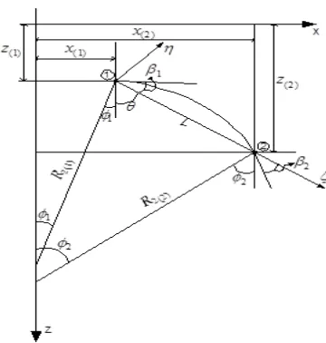
The geometrical variables of the element are determined as polynomials in terms of these normalized co-ordinates and their derivatives (η’ and η”). Referring to the Figure 3, the geometrical variables are; “s” is the arc length of the element, x and z represent the global coordinates of the strip, “R1” is the radius of curvature of the curved strip,
“R2” is the circumferential radius of curvature, “
φ
” is theslope angle of the curved strip, and “β” is the slope angle of the substitute curve with respect to its local co-ordinates. From Figure 3:
2 1 2 1 2 1 2 tan 1 cos
− ′ + = − +
=
β η
β
− ′ + ′
≈ 4...
8 3 2 2 1
1 η η (14)
ζ η ζ
βd L d
L
ds 2
1 2 1
cos
+ ′
= =
ζ η
η d
L
+ ′ − ′
≈ 4...
8 1 2 2 1
1 (15)
Where L is the chord length of the element.
(
sinθ
)
ζ
(
cosθ
)
η
1 L L
x
x= + + (16)
Where x1 is the distance co-ordinate of node (1), θ is the
angle between the element chord and the longitudinal axis. ′== φβ=
{
θ(
θ++(
β)
θ)
η′}
cos sin cos
sin cos x
≈ − η′ + η′
{
θ+(
θ)
η′}
cos sin ... 4 8 3 2 2 1 1
(17)
=sinφ=cosβ
{
cosθ−(
sinθ)
η′}
r x
≈ − η′ + η′
{
θ−(
θ)
η′}
sin cos ... 4 8 3 2 2 1
1 (18)
The arc length “s” is determined by integrating (ds) and the arc length of the element (l) is evaluated as follow:
∫ + ′ − ′
= ∫
=
1
0
... 4 8 1 2 2 1 1 1
0
ζ η
η d
L s
s ds
l (19)
3. Results and Discussion
The validity of the Mixed formulation of Curved Finite Strip element (MCFS) and the accuracy of results are demonstrated by one numerical example of cylindrical shell with simply supported at the curved edges (longitudinal direction) and free along the straight edges (transverse direction) and it is subjected to a loading of
q = 90 Ib/ft2. The thickness of the shell is 3 inches and the radius of curvature is 25 feet while the length of the straight edge is 50 feet.Details of the shell geometry and material properties are given below in Figure 6.
The results obtained from the (MCFS) were compared with the Shallow Shell Theory(SST) solutionpresented by Scordelis [10].
E = 3 x 10⁶psi, ν = 0.0, h = 3 in., R = 25 ft., a = 50 ft., ϕ i = - 40o and ϕ f = 40o
Figure 6: Details of the shell geometry and material properties.
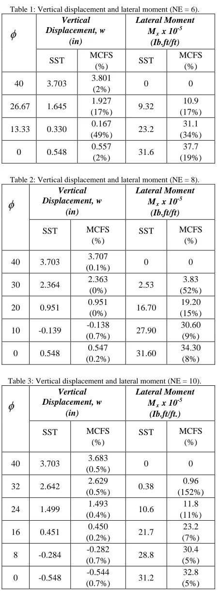
Convergence is investigated by changing the number of strip elements (NE). The cylindrical shell is discretized into six, eight and ten longitudinal strip elements while the shape mode remains equal to one. Due to symmetry, only the results of the half shell are presented. The results of the vertical displacement (w) and the lateral moment (Mx) obtained by (MCFS)
Table 1: Vertical displacement and lateral moment (NE = 6).
φ
Vertical Displacement, w
(in)
Lateral Moment Mx x 10
-5
(Ib.ft/ft)
SST MCFS
(%) SST
MCFS (%)
40 3.703 3.801
(2%) 0 0
26.67 1.645 1.927
(17%) 9.32
10.9 (17%)
13.33 0.330 0.167
(49%) 23.2
31.1 (34%)
0 0.548 0.557
(2%) 31.6
37.7 (19%)
Table 2: Vertical displacement and lateral moment (NE = 8).
φ
Vertical Displacement, w
(in)
Lateral Moment Mx x 10-5
(Ib.ft/ft)
SST MCFS (%)
SST MCFS (%)
40 3.703 3.707
(0.1%) 0 0
30 2.364 2.363
(0%) 2.53
3.83 (52%)
20 0.951 0.951
(0%) 16.70
19.20 (15%)
10 -0.139 -0.138
(0.7%) 27.90
30.60 (9%)
0 0.548 0.547
(0.2%) 31.60
34.30 (8%)
Table 3: Vertical displacement and lateral moment (NE = 10).
φ
Vertical Displacement, w
(in)
Lateral Moment Mx x 10-5
(Ib.ft/ft.)
SST MCFS (%)
SST MCFS (%)
40 3.703 3.683
(0.5%) 0 0
32 2.642 2.629
(0.5%) 0.38
0.96 (152%)
24 1.499 1.493
(0.4%) 10.6
11.8 (11%)
16 0.451 0.450
(0.2%) 21.7
23.2 (7%)
8 -0.284 -0.282
(0.7%) 28.8
30.4 (5%)
0 -0.548 -0.544
(0.7%) 31.2
32.8 (5%)
As we can see from the results in Tables 1, 2 and 3, when the shell is modeled by 6 longitudinal strip elements (i.e. NE = 6), the vertical displacements obtained by (MCFS) are higher than those calculated by (SST) solution. The maximum difference in the results of vertical displacements is 49%. The results converge quickly when more strip elements (i.e. NE = 8 and 10) are used, where the maximum difference in the results of vertical displacements becomes 0.7%. A slight improvement in the results of the vertical displacements can be observed when the number of the longitudinal strip elements are 8 and 10. The maximum difference in the results of the lateral moment is high for the mesh with 6 strip elements, i.e. 34%. The moment converges slightly to 15% and 11% when the number of strip elements is increased to 8 and 10 respectively. The convergence of the maximum moment at the center of the shell is improved from 19% to 5%. However, the value of the moment increased to 52% higher than the (SST) solution at the strip near the longitudinal free edge. Similar observation can be made for the mesh with 10 strip elements, where the difference (%) in this mesh can be as high as 152% in the strip near the longitudinal free edge (i.e. ϕ = 32o). For this particular example, the results of the moments are converged as they moved away from the free edge.
4. Conclusion
The numerical example shows, in general, the validity of the mixed finite strip formulation to analyze cylindrical shells. The results of the vertical displacements and moments are found to be in agreement when compared with the shallow shell theory solution.
References
[1] Herrmann, L. R., Finite element bending analysis of plates, Proc. ASCE, J. Eng. Mech. Div., vol. 93, EM5, pp. 13-26, 1967.
[2] Connor, J., Mixed models for shells, Finite element techniques in structural mechanics, Tottenham and Brebbia. University of Southampton, U. K., 1970.
[3] Prato. C., Shell finite element method via Reissner's principle, Int. J. Solids structures, vol.5, pp. 1119-1133, 1969.
[4] Elias, Z., Mixed finite element methods for axisymmetric shells, Int. J. Num. Methods Eng., vol. 4, pp. 261-277, 1972.
[5] Gould, P. and Sen, S.K., Refined mixed finite element for shells of revolution, Proc. Third Conf. On matrix methods in structural mechanics, Wright-Patterson. AFB, Ohio, 1971.
formulation, Int. J. Num. Meth. Eng., vol. 10, 1978, pp. 861-872.
[7] Cheung Y. K., Finite Strip Method in Structural Analysis, 1st ed., Pergamum Press, 1976.
[8] Abdunnaser M. Younes, Finite Strip Method – A comparative study between the stiffness and the mixed approaches, M.Sc. Thesis, Al-Fatah University, Libya, spring 1996.
[9] Tuhami A., Analysis of Cylindrical Shells Using Mixed Formulation of Curved Finite Strip Element, M. Sc. Thesis, University of Tripoli, 2007.