Adaptive Optimal LQ Regulator for Linear Systems Applied to Discrete Power System Model

Adaptive Optimal LQ Regulator for Linear

Systems Applied to Discrete Power System

Model

E.S. Sergaki1, A.K. Boglou2, D.I. Pappas3, A.G. Arvanitakis4

School of Electrical & computer Engineering, Technical University of Crete, Chania, Greece1

Department of Petroleum and Mechanical Engineering, Eastern Macedonia and Thrace, Kavala, Greece2,3

Electrical Engineering, of the Industrial and Energy Application, Thessaloniki, Greece4

ABSTRACT: The proposed control strategy of this paper solves the adaptive LQ optimal regulation problem for

continuous-time systems, by the utilization of, a new class of multirate controllers, called TPMCs (two-point-multirate controllers). In this type of controller, the control is constrained to a certain piecewise constant signal, and the controlled plant output is detected many times over a fundamental sampling period. The adaptive control strategy suggested here relies on solving the continuous LQ regulation problem. On the basis of this strategy, the original problem is reduced to an associate discrete-time LQ regulation problem for the performance index, with cross-product terms, for which a fictitious static-state feedback controller needs to be computed. The present technique essentially resorts to the computation of simple gain controllers rather than to the computation of state observers, as compared to other known techniques. The proposed adaptive scheme is readily applicable to non-minimum phase systems and to systems that do not possess the parity interlacing property (i.e., they are not strongly stabilizable). The discrete linear open-loop system model under consideration derived from the associated continuous 3th-order linearized open-loop model of an actual working power system, consisting by an 160 MVA synchronous generator and supplying power to an infinite grid, through a step-up transformer and its adequate transmission line. Through the obtained pertinent simulation results, the validity and practical usefulness of this design technique is fully assessed.

KEYWORDS: Adaptive Control, optimal multirate control , LQ regulator, parameter estimation, power system.

I. INTRODUCTION

coefficients. Therefore, just as single-rate controllers, the multi-rate controllers do not violate the finite memory constraint of the microprocessors. In particular, the control strategy presented here is essentially a combination of the control strategies reported in [11,10]. The control is constrained to a certain piecewise constant signal, while the controlled plant output is detected many times over a fundamental sampling period. The proposed adaptive control strategy relies on solving the continuous LQ regulation problem.

In the present work, the adaptive optimal LQ regulator via a TPMRC scheme is used, to design a desirable excitation controller for a turbogenerator system [14,15], in order to enhance its dynamic stability characteristics. The particular turbogenerator studied in this paper is a 160 MVA unit with excitation voltage, supplying power to an infinite grid via a step-up transformer and a high-voltage transmission line.

The design of the digital controller, which leads to the associated discrete closed-loop control system, in order to achieve the enhanced dynamic stability characteristics, is accomplished by properly applying the presented adaptive optimal LQ regulator, by using the TPMRCs technique.

II. PRELIMINARIES AND PROBLEM FORMULATION

Consider the continuous-time, linear time-invariant single-input, single-output system described in state space by the

following equations:

( )t  ( )t B ( )t

x Ax u , (1a)

( )t  ( )t

y Cx (1b)

where ( )xt Rn, ( )ut R andy( )t R are the state, control and output signals, respectively and A, B, C, D are real matrices having appropriate dimensions. With regard to system (1), we make the following assumption [2,9].

Assumption 1. System (1) is controllable (can be stabilized), observable (can be detected), and of known order n. The

following definition will be useful in the sequel.

Definition 1. The generalized reachability Grammian? of order N on the interval [0, To] is defined as:

1 1

N 0

0

(Τ ,0)=Τ

N T

N  



 

 





W where: 0_, ˆ(N 1) ˆ

N c

T T

N

 



  



  A Β ,

0

ˆ _{exp( ),} ˆ N_{exp( )}

N T

c TN T 



A A B A B

Let pN be the rank of WN(TO, 0). As WN(TO,0)



matrix Bn such that:

( ,0)

T

n N  N To

B B W (2)

The input of the plant is constrained to the following piecewise constant control:

1

ˆ ˆ

( ) ( ) T r ( )

o N o N N o

kT T  _ kT T_ kT

    u  B u , ˆ( ) pN o

u kT 

for t = kT0 + μTN + ζ; μ = 0,1,... , n — 1; k



The output of the plant is detected at every TM = To/M, such that:

( ) T ( )

o M o M

y kT T c x kT T (3)

where MZ_{is the output multiplicity of the sampling.}

plant input and output may be performed at a different rate.

The sampled values of the plant output obtained over [kT0, (k + 1)T0) are stored in the M-dimensional column vector

ˆ (kTo)

γ of the form:

(4)

The vector γˆ (kTo)is used in the control law of the form:





ˆ (k1)To  uˆ(kTo) (kTo)

u L u Kγ (5)

, .

NxM NxM

p p

u  

L K where:

The adaptive LQ regulation problem treated in the present work can be presented as the following:

Find a TPMRC (Two-point-multirate controller), that, when applied to system 1, minimizes the following cost criterion

[1,2]:

2 2

0 1

( ( ) ( )) 2

J qy t ru t dt





_

where, for the design constants q and r, we have q0, r0 and ( , T)

qcc

Α is an observable pair.

III. SOLUTION OF THE LQ OPTIMAL REGULATION PROBLEM APPROPRIATE FOR THE ADAPTIVE CASE

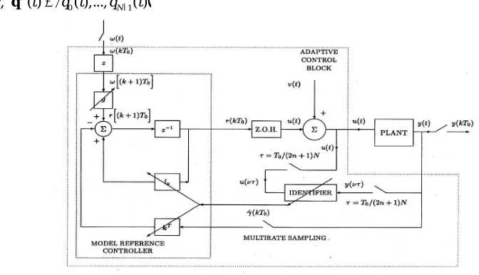
In order to obtain a valid solution for the aforementioned TPMRC-based LQ optimal regulation problem, that will be more appropriate for application to systems with unknown parameters, we slightly modify our control strategy as shown in fig 1. In particular, we introduce in the control loop the persistent excitation signal υ(t), which is defined as [6,7,8]:





( )t T( ) ,t T( )t q t( ),...,qN ( )t

 q v q  _ (7)

Fig. 1 The structure of the adaptive control system.

Here, q(t) is the TN-periodic vector function with elements having the form:





,

( ) , ( 1) ,

i i N N

q t q for t T  T i=0, 1,…,N-1, μ=0, 1,…,N-1 (8)

where q is a constant taking the following values:







It is pointed out that v is as yet unknown. We remark that the additive term ( ) T( ) , t q t v

  in the input of the continuous-time system is used only for identification purposes and, as it will be shown later, it is selected so as not to influence the LQ regulation problem.

In the sequel, the nature of the control law Eq. 5 will be explained. To this end, we establish the following fundamental theorems.

Theorem 3.1. The following basic formula of the multirate-output sampling mechanism holds [8,9]:





Hx γ Du , (10)

where _{H }Mxn _{andD }MxpN _{have the following forms:}

1 0 1 1 1 1 1 ˆ ˆ ( ) ˆ ( ) . . , . . . . ˆ T T M T T M T T M                                          _ _   c B c A c B c A Η D c B c A

, where: _ˆ * _{( ) ˆ} M _{, 0,1,..., 1.}

M N M



  



   

B B A B (10)

Using the above definitions and after algebraic manipulation, the matrix gain K will obtain the following form [11]:









ˆ

T T T

N N N N N

 _

 

_   _

 

K R B PB G B PΦ H 0 E (11)

Furthermore, the matrix gain Lu will obtain the form [11]:









1 1 ˆ

T T T

u N N N N N

 _

 

  

 

 

L R B PB G B PΦ Η 0 ED, (12)

where Φ=exp(ATo) and P is the symmetric positive-definite solution of the discrete algebraic Riccati equation [1,5].

Note that, in this case, another solution for the matrix pair (K, Lu) is given, by:









N N N N N



  

K R B PB G B PΦ H , (13)









u N N n N N





  

L R B PB G B PΦ H D (14)

Where H1 is the left pseudoinverse of matrix H, that is, the matrix fulfilling the condition H1H = I. The resulting discrete closed-loop system matrix (Acl d/ ) takes the following form:

/ /

cl d  ol d N

A A B KH, where cl=closed-loop, ol=open-loop and d =discrete.

IV. DESIGN AND SIMULATIONS OF RESULTING DISCRETE CLOSED-LOOP POWER SYSTEM MODEL

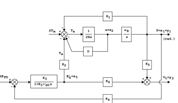
The power system under study fig 2 [14,15], consists of a 160 MVA turbogenerator with constant excitation voltage EFD, supplying power via a step-up transformer and a high-voltage transmission line to an infinite grid. The numerical

Fig. 2 Simplified representation of investigated practical power system.

Based on the state variables presented in fig. 2 and the values of the parameters and the operating point (see Appendix A), the system of fig. 2 can be described in a state-space form, as in the form of system 1, where:

T q

E

  

    

x , u 









T t

v





y

The numerical values of the matrices A, B and C are given in Appendix A.

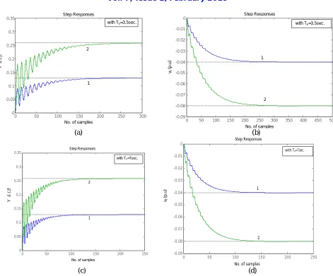
The eigenvalues of the original continuous open-loop power system models and the simulated responses of the output variables (δ, ω, vt), are presented in Table I and fig. 3, respectively.

Table I. Eigenvalues of original continuous open-loop power system models.

Original open-loop power system model λ

-0.2723+6.2253i -0.2723-6.2253i

-0.1889

The associated computed discrete linear open-loop power system model, based on the above transformed linearized continuous open-loop system model, is given in Appendix B. The fundamental sampling period To is selected for the

two cases as:

case a) To =3.5 sec. and case b) To=7 sec.

The computed magnitude of the eigenvalues of the discrete open-loop power system models and the simulated responses of the output variables (δ, vt), (for both the above two cases), are shown in Table II and fig. 3, respectively.

Table II. Magnitude of eigenvalues of discrete original open-loop and designed closed-loop power system models.

Original open-loop power system

model



To=3.5sec. 0.9731 0.9731 0.9813

To=7sec. 0.9470 0.9470 0.9629

Designed closed-loop power

system model



ˆ

To=3.5sec. 0.3600 0.1563 0.1563

To=7sec. 0.2906 0.2906 0.0333

(a) (b)

(c) (d)

Fig. 3 (a), (b), (c), (d): Simulation results represent the responses (δ, vt) of the discrete response system: (1), (2): for the

open loop to step input power load charges ΔΤm=0.05p.u. (ΔΕFD=0.0p.u.) and ΔΤm = 0.10p.u. (ΔΕFD=0.0p.u.)

respectively.

In the present simulation, our control objective is to solve the problem of minimizing the performance index Eq. 6, using the selected weighing matrices (for the above two cases):

q=3.5 and r=1.

The K and Lu feedback matrices were computed as:

for case a):

1.2633 1.5695 1.5 1.0139 0.5481 0.0622 1.9469 1.7262 1.7556

             K ,

0.5081 0.0581 0.1408 0.1272 0.4092 0.0040 0.4589 0.1898 0.0878 u                L

and for case b):

0.4652 0.1886 0.1108 0.0696 0.3163 0.0643 0.0918 0.3285 0.6437

            K ,

0.1035 0.3467 0.0704 0.1688 0.2406 0.0089 0.0043 0.5300 0.2652

u                L

0 50 100 150 200 250

-0.09 -0.08 -0.07 -0.06 -0.05 -0.04 -0.03 -0.02 -0.01 0 Step Responses

No. of samples

vt

(p

.u

)

with To=7sec.

2 1

0 50 100 150 200 250

0 0.05 0.1 0.15 0.2 0.25 0.3 0.35 Step Responses

No. of samples

δ

(

ra

d

.)

with To=7sec.

2

1

0 50 100 150 200 250 300 350 400 450 500

-0.09 -0.08 -0.07 -0.06 -0.05 -0.04 -0.03 -0.02 -0.01 0 Step Responses

No. of samples

with To=3.5sec.

1

2

0 50 100 150 200 250 300

0 0.05 0.1 0.15 0.2 0.25 0.3 0.35 Step Responses

No. of samples

δ

(

ra

d

.)

with To=3.5sec.

We select (for both two cases a) and b)) the input and the output multiplicities of the sampling, such as: M = N =5. Finally the nominal parameter vector θ has the form [10,12]:

for case a): θ 





for case b): θ 





The numerical values of the matrices referring to the discrete closed-loop power system models of the above two cases are not included here, due to space limitations.

The simulation results for the discrete open-loop power system models and for the closed-loop power system models (i.e.: eigenvalues, eigenvectors, Riccati solutions, responses of system variables etc.), for zero initial conditions and with input disturbances (ΔTm=0.05 & ΔTm=0.10), were obtained using special software, based on the theory of §( I,II)

and implemented as a typical m-file, running in a MATLAB® environment.

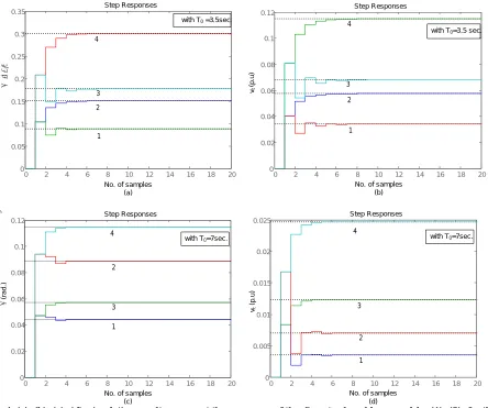
The responses of the output variables (δ, vt) of the designed closed-loop power system models, for zero initial

conditions and unit step input disturbance, are shown in fig. 4.

Fig. 4 (a), (b), (c), (d): simulation results represent the responses of the discrete closed-loop models: (1), (2): for the two closed-loop, to step input power load changes ΔTm=0.05 p.u. (ΔEFD=0.0 p.u.) and ΔTm=0.10 p.u. (ΔEFD=0.0 p.u.)

respectively, (3), (4): for the two closed-loop to step input power load changes ΔTm=0.05 p.u. (ΔTm=0.0 p.u.) and ΔTm=0.10 p.u. (ΔTm=0.0 p.u.) respectively.

0 2 4 6 8 10 12 14 16 18 20

0 0.005

0.01 0.015 0.02

0.025 Step Responses

No. of samples (d) vt

(p

.u)

with T0=7sec.

4

3

2

1

0 2 4 6 8 10 12 14 16 18 20

0 0.02 0.04 0.06 0.08 0.1

0.12 Step Responses

No. of samples (c)

δ

(rad.

)

with T0=7sec.

4

2

3

1

T0

0 2 4 6 8 10 12 14 16 18 20

0 0.02 0.04 0.06 0.08 0.1

0.12 Step Responses

No. of samples (b)

with T0=3.5 sec.

4

3

2

1

0 2 4 6 8 10 12 14 16 18 20

0 0.05 0.1 0.15 0.2 0.25 0.3

0.35 Step Responses

No. of samples (a)

δ

(rad.

)

with T0 =3.5sec.

1 2 3 4

vt

(p

From fig. 4 it is clear that the dynamic stability characteristics of the designed discrete closed-loops models are far more superior than the ones of the original open-loop model, which further attests in favor of the proposed adaptive LQ-TPMRCs-control technique.

V. CONCLUSION

An efficient control strategy based on two-point multirate controllers has been presented in order to solve the continuous adaptive LQ regulation problem for linear systems and in order to design a desirable excitation controller for an hydrogenerator system, so to enhance its dynamic stability characteristics. The proposed adaptive control scheme offers acceptable closed-loop response as well as more design flexibility, particularly in the cases where the system states are not measurable and system’s performance is at least comparable to known LQ optimal regulation methods. The clear simplicity of the TPMRCs used, makes them an appropriate and reliable tool for the design of such implementable controllers.

REFERENCES

[1] Ogata, K. “Discrete time control systems”, Englewood Cliffs, N. J: Prentice-Hall, 1987.

[2] Hagiwara T., Araki M., “Design of a stable state feedback controller based on the multirate sampling of the plant output”, IEEE

Transactions. Autom. Control, AC-33, pp.812-819, 1988.

[3] Er M.-J., Anderson B.D.O., “Practical issues in multirate-output controllers”, Int. J. Control, vol. 53, No. 5, pp.1005-1020, 1991.

[4] Al-Rahmani H.M., Franklin G.F, “A new optimal multirate control of linear periodic and time-invariant system”, IEEE Transactions, Autom.

Control AC-35, 406–415, 1990.

[5] Sun J., Ioannou P., “Robust adaptive LQ control schemes”, IEEE Transactions, Autom. Control AC-37, pp.100–106, 1992.

[6] Tsao T., Hutchinson S., “Multi-rate Analysis and Design of Visual Feedback Digital Servo-Control”, Journal of Dynamic Systems

Measurement and Control, vol. 116, no. 1, pp. 45-55, 1994

[7] Janardhanan S., Bandyopadhyay B., “Multirate Output Feedback Based Robust Quasi-Sliding Mode Control of Discrete-Time Systems”,

IEEE Transactions on Automatic Control, vol. 52, No. 3, pp.499-503, 2007.

[8] Narendra K. S., Annaswamy A.M., “Stable Adaptive Systems”, Englewood Cliffs, NJ: Prentice Hall, 1989: Dover Publications 2004.

[9] Tao G., “Adaptive Control Design and Analysis”, Hoboken, NJ: Wiley-Interscience, 2003.

[10] Arvanitis K. G., “An Indirect Model Reference Adaptive Control Algorithm Based on Multidetected-Output Controllers”, Appl. Math. And

Comp. Sci., vol. 6, No. 4, pp.667-706, 1996.

[11] Arvanitis K. G., “A New Adaptive Optimal LQ Regulator for Linear Systems Based on Two-Point-Multirate Controllers”, Control and

Intelligent Systems, vol. 28, No. 1, pp.1-18, 2000.

[12] Arvanitis K .G.,”A New Multirate LQ Optimal Regulator for Linear Time-Invariant Systems and its Stability Robustness Properties”,

International Journal of Applied Mathematics and Computer Science, vol. 8, pp.101-156, 1998.

[13] Hassan S., Li H., Kamal T., Arifoğlu U., Mumtaz S., Khan L., “Neuro-Fuzzy Wavelet Based Adaptive MPPT Algorithm for Photovoltaic

Systems”, Energies, vol. 10, no. 3, pp.394, 2017.

[14] Papadopoulos D.P., Boglou A.K., “Turbogenerator-System Controller design via exact model-following techniques”, INT. J. Systems Sci.,

vol. 18, No. 12, pp. 2239-2247, 1987.

[15] Smith J. R., Papadopoulos D.P., Cudworth C. J., Penman J., “Prediction of Forces on the Retaining Structure of hydrogenerator During

Severe Disturbance Conditions”, Electric Power Systems Research, vol. 14, pp.1-9, 1988.

Appendix A

Numerical values of the system parameters and the operating point (p.u. values on generator ratings).

Turbogenerator: Operating point:

160 MVA, 2-pole, pf= 0.894, xq=1.7, xq=1.6,

x'd=0.245p.u. '

0 d



P0=1.0, Q0=0.5, EFDo=2.5128, Eqo=0.9986, Vt0=1.0,

Tmo=1.0p.u.; δ0=1,1966rad; K1=1,1330, K2=1.3295,

K3=0.3072, K4=1.8235, K5=-0,0433, K6=0.4777.

External system:

Appendix B

Numerical values of matrices A, B, C, of the original continuous 3th –order system:

0 377 0

0.1030 0.1818 0.1209 0.3091 0 5.5517

     _   _      A , 0 0 0.0909 0 0 0.1695     _{ }    

B , 1 0 0

0.0433 0 0.4777

 

 _ 

 

C

Appendix C

Constant matrices of discrete open-loop power system model, based on figs. 1 and 2 with:

a)sampling period To = 3.5 sec.

/

0.8154 35.0092 0.2153 0.0094 0.7985 0.0109 0.0282 0.5505 0.9486

ol d       _  _    

A , /

0.1649 0.0084 0.0017 ol d     _{ }    

B , Col d/ C.

/

0.8281 1.0242 0.8777 2.1548 2.3675 1.9064

1.2109 1.2098 0.8826

cl d               



A

2.0865 0 0

3.8912 0.9189 0 1.8755 0.9712 0.1432

cl d   _        



B

b) sampling period To = 7 sec.

/

0.3422 56.6199 0.7618 0.0148 0.3149 0.0170 0.0445 1.9477 0.9118

ol d    _{ }        



A

0.5953 0.0137 0.0126 ol d          



B

/

0.1564 0.0570 0.1638 0.2484 0.0871 0.1673

0.0162 0.2456 0.0134

cl d      _{ }        



A

0.9411 0 0

1.0240 1.1229 0 0.4352 1.3529 0.5154

cl d   _        

