Computer-aided detection of colonic polyps with level set-based adaptive convolution in volumetric mucosa to advance CT colonography toward a screening modality

(1)

O R I G I N A L R E S E A R C H

Computer-aided detection of colonic polyps

with level set-based adaptive convolution

in volumetric mucosa to advance CT colonography

toward a screening modality

Hongbin Zhu1 Chaijie Duan1 Perry Pickhardt2 Su Wang1

Zhengrong Liang1,3 1_{Department of Radiology,} 3_{Department of Computer Science,}

State University of New York, Stony Brook, NY, USA; 2_Department

of Radiology, University of Wisconsin Medical School, Madison, WI, USA

Correspondence: Zhengrong Liang Department of Radiology, State University of New York at Stony Brook, Stony Brook, NY 11794, USA

Tel +1 631 444 7837 Fax +1 631 444 6450 Email [email protected]

Abstract: As a promising second reader of computed tomographic colonography (CTC) screening,

the computer-aided detection (CAD) of colonic polyps has earned fast growing research interest. In this paper, we present a CAD scheme to automatically detect colonic polyps in CTC images. First, a thick colon wall representation, ie, a volumetric mucosa (VM) with several voxels wide in general, was segmented from CTC images by a partial-volume image segmentation algorithm. Based on the VM, we employed a level set-based adaptive convolution method for calculating the fi rst- and second-order spatial derivatives more accurately to start the geometric analysis. Furthermore, to emphasize the correspondence among different layers in the VM, we introduced a middle-layer enhanced integration along the image gradient direction inside the VM to improve the operation of extracting the geometric information, like the principal curvatures. Initial polyp candidates (IPCs) were then determined by thresholding the geometric measurements. Based on IPCs, several features were extracted for each IPC, and fed into a support vector machine to reduce false positives (FPs). The fi nal detections were displayed in a commercial system to provide second opinions for radiologists. The CAD scheme was applied to 26 patient CTC studies with 32 confi rmed polyps by both optical and virtual colonoscopies. Compared to our previous work, all the polyps can be detected successfully with less FPs. At the 100% by polyp sensitivity, the new method yielded 3.5 FPs/dataset.

Keywords: colonic polyps, level set, adaptive convolution, middle-layer enhanced integration,

volumetric mucosa, support vector machine, computer-aided detection, CT colonography

Introduction

According to the American Cancer Society statistics, colorectal carcinoma is the third most commonly diagnosed cancer and the second leading cause of death from cancer in the United States (see http://www.cancer.org/docroot/home/index.asp).1_{It was}

estimated that 154,000 new cases would be diagnosed with 52,000 dying from the disease in 2007. Fortunately, most colon cancer probably arises from polyps, which can take 5–15 years for malignant transformation. Thus, early detection and removal of small polyps of less than 10 mm will effectively decrease the incidence of colonic cancer.2–4_{As a new minimally-invasive screening technique, computed tomographic}

colonography (CTC) or CT-based virtual colonoscopy (VC) has shown several advantages over the traditional optical colonoscopy (OC),5_{and an annual screening}

is recommended for people over 50 years old. In order to improve the sensitivity and consistency of CTC in the identiﬁ cation of polyps, computer-aided detection of polyps (CADpolyp) has been suggested as an effective second reader assisting radiologists for ﬁ nding polyps in the colon.6–8

Cancer Management and Research downloaded from https://www.dovepress.com/ by 118.70.13.36 on 20-Aug-2020

(2)

Zhu et al

Typical polyps appear as protrusions out of the colon wall into the lumen. Therefore, in state-of-the-art CAD systems, the colon wall is ﬁ rstly segmented from the original three-dimensional (3D) CTC image, followed by a shape analysis on the colon wall to generate initial polyp candidates (IPCs). Finally, various learning methods are used to reduce false positives (FPs).9

As the very ﬁ rst step of a CAD system, colon wall segmen-tation explicitly or implicitly determines the overall detection performance via the successive shape analysis. In this study, we employed a soft segmentation method10_{to extract the colon}

wall as a volumetric mucosa (VM) with a thickness of several voxels, which is considered to be a complete representation of the colon wall without any artiﬁ cial shrinkage and enlargement. Unfortunately, the relatively-thick VM often appears blurred and noisy, so we employed an anisotropic diffusion ﬁ lter to smooth the VM. More details about the VM extraction and smoothing are referred to in the section on Volumetric mucosa extraction, below. Upon the extracted colon wall, polypoid-like initial candidates are determined by thresholding the geometric measurements, such as the mean curvature and sphericity ratio,11_{the shape index and curvedness,}12,13_the

convexity or concavity,14_{and the surface normal overlap.}15

All these geometric measurements are functions of the ﬁ rst- and second-order spatial derivatives of the 3D CTC images. Monga and colleagues16_{convoluted the 3D image volume}

with derivatives of Gaussian kernels (the 3D Deriche ﬁ lters17₎

to compute the derivatives. Thirion and colleagues18_{just used}

a central differencing scheme to calculate the derivatives but after ﬁ ltering the 3D image with a Gaussian kernel. However, the robustness and effectiveness of both methods highly depend on the kernel window size (decided by the parameters of α₁ and

α2 in Monga’s method, and σ in Thirion’s method) they used.

Therefore, Campbell and Summers19_{explored the optimal}α 1

and α₂ based on several phantoms, and they found that even with those optimal parameters, spurious computations could be observed on thin ﬂ at folds, caused by the interference of different topological structures residing in the same kernel window. To address such a problem, Huang and colleagues20

and Sundaram and colleagues21_{built a geometric surface}

repre-sentation of the colon wall instead of the often used volumetric voxel representation, and shape analysis was conducted only on the surface. With the assumption that the surface is accurately extracted from the 3D CTC image, the interference between different topological structures can be avoided. However, Wijk and colleagues22_{employed the normalized convolution to}

calculate the ﬁ rst- and second-order spatial derivatives, where the different structures were differentiated by using the gradient

of a distance transform23_{based on the air-tissue interface. The}

mathematically sophisticated method used by Wijk and col-leagues22_{is time consuming, and the hard segmented air-tissue}

interface cannot reﬂ ect the partial volume effect (PVE). Simi-larly, Wang and colleagues24_{directly eliminated the contribution}

of voxels of different structures in the convolution by Deriche.17

However, the single-voxel interface layer (referred to as the starting layer (SL) in the following text) used to build up the distance transform was not properly selected either, and due to PVE, their SL would overlook the polypoid structures and incorrectly synthesize nonexisting polypoid structures. The details of this will be addressed in the level set-based adaptive convolution (LSAC) method discussed below. In this study, we employed a LSAC method to calculate the partial derivatives. As such, a more accurate and robust SL was retrieved.

Geometric features aforementioned to characterize colonic polyps have been extensively presented towards CADpolyp. However, most of them were extracted based on a single layer mucosa representation. Necessity still exists for exploring the correspondence among different layers of the mucosa/colon wall in CTC images. Wang and colleagues25_introduced

“global” versions of the shape index and curvedness, within spatial domain, by linear smoothing along the principal direc-tions. Nevertheless, their method ignored the correspondence between different layers of the mucosa/colon wall. Therefore, Wang and colleagues24_{smoothed the ﬁ rst and second principal}

curvatures along the normal direction, referred to as weighted integral curvature along normal directions (WICND). In their method, the voxels on the middle-layers of the VM were treated equally as those voxels on the other layers. However, we argue that the middle-layers of the mucosa/colon wall appear smoother, and should be more reliable than the other ones when conducting shape analysis. In this study, we intro-duced a middle-layer enhanced integration (MEI) strategy to reﬁ ne the geometric features, where higher weights were put on the voxels at the middle layers of the VM.

The remainder of this paper is organized as follows. In Methodology, we ﬁ rstly provide a brief overview of the proposed CAD scheme, and then the aspects of the pipeline are demonstrated, especially the LSAC method. We then describe the performance evaluation and give the results. Finally, some conclusions are drawn.

Methodology

Overview

The whole CAD pipeline can be outlined in four stages: VM extraction, IPC detection, FP reduction and detection presentation, as shown in Figure 1.

(3)

Computer-aided detection of colonic polyps

In the ﬁ rst stage (to be detailed in Volumetric mucosa

extraction, below), through the MAP-EM (maximum a

posteriori expectation maximization) soft segmentation algorithm,10_{the mixture percentage of each tissue type inside}

each voxel in the CTC images was estimated, from which the VM was extracted and smoothed afterward. In Stage 2 (to be detailed in The level set-based adaptive convolution (LSAC) method, The middle-layer enhanced integration (MEI) strategy, and Polyp candidate extraction, below), we ﬁ rstly applied the LSAC method inside the VM to conduct the geometric computation. The computed geometric measures were then smoothed by the MEI strategy and used to extract suspicious patches. The suspicious patches were fed to the ﬁ lter25_to

remove noise-induced patches. In what follows, the survived patches grew into the tissue area25,26_{to form the IPCs. In the}

third stage (to be detailed in FP reduction, below), both shape

and textural features were extracted for each IPC, and fed into a weighted SVM model27_{to reduce FPs. In the last stage, the}

detection results were displayed in a CTC commercial system and presented to physicians to serve as second opinions (to be detailed in Detection presentation, below).

Volumetric mucosa extraction

For any imaging modality (eg, CT), PVE always exists. Considering the use of positive-contrast tagging agents to opacify the residual fecal for differentiation of the materi-als from colon wall and polyps,28_{PVE became severe and}

the thickness of the VM varied dramatically. In the case of extracting mucosa for CAD in CTC, a sheer surface ignoring PVE, as segmented by most of the previous colon-wall seg-mentation algorithms, undoubtedly shrunk or even distorted the true mucosa without any chance of recovery. Figure 2

Feature extraction

SVM classification

Stage 3: FP reduction

Detection result presentation

Stage 4: Detection presentation

CTC images

MAP-EM segmentation

Extraction of VM

Stage 1: VM extraction

LSAC in the VM

Extraction of IP Cs

Stage 2: IPC detection

MEI smoothing

Figure 1 Pipeline of the presented CADpolyp system.

Abbreviations: CTC,computed tomographic colonography; FP, false positive; IPC, initial polyp candidate; LSAC, level set-based adaptive convolution; SVM, support sector machine; VM, volumetric mucosa.

a) b) c) d)

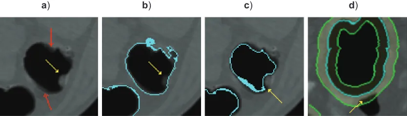
Figure 2 Segmented colon walls by traditional hard segmentation algorithms: a) part of an original CTC image slice, the red arrow indicates the blurring area near the air-colon interface refl ecting the PVE and the yellow arrow fl ags a 9 mm polyp; b) the colon wall (the cyan curve) in another slice near the same polyp in a) was created by region growing to -300 HU,11_{which cuts off part of the polyp in light gray indicated by the yellow arrow;}_c_{) the colon wall (the cyan curve) of the same slice in}_a_{) was created by region growing}

to -800 HU,11_{where the polyp gets enlarged near the yellow arrow; and}_d_{) a thickened colon wall (the area between the two green curves) was created by morphologically}

dilating the iso-surface at -650 HU (the cyan curve) inward and outward by 5 mm,12_{where the yellow arrow indicates that part of the small bowel is incorrectly included.}

Abbreviations: CTC,computed tomographic colonography; PVE, partial volume effect; VM, volumetric mucosa.

(4)

Zhu et al

fully illustrates the limitation of such hard thresholding segmentation without considering PVE. Although by locally adjusting the threshold for a better colon wall representation with less possibilities of shrinkage or enlargement (ie, by a particular threshold value), it was still data-oriented and hardly to be generalized to all the cases. More speciﬁ cally, the over-ﬁ tted colon wall12_{may include noncolonic structures}

with increased FP rates, as shown in Figure 2d. Furthermore, a large amount of unwanted air and tissue areas may also be included, resulting in an increased computational burden.

To address the PVE, a soft image segmentation algo-rithm10_{was developed. The algorithm aims to estimate the}

tissue mixture percentages inside each voxel within the framework of iterative MAP-EM estimation. By viewing the tagged fecal material as an extra class type, its mixture fractions inside each voxel could be accurately estimated and cleansed by assigning them to those of air class. The output of the MAP-EM algorithm includes: (1) an electronically cleansed image I_T in CT densities (Figure 3b); and (2) the colon lumen (air class) percentage distribution map in the range of [0, 1], I_L, to reﬂ ect the PVE (Figure 3c). Finally, the VM with variable thickness was obtained by directly extracting those voxels whose colon percentages are between 0 and 1, which means that they are not fully occupied by either tissue or air (Figure 3d). Compared to the sheer surfaces of Figure 2b and Figure 2c via the traditional hard thresholding segmentation, the extracted VM of Figure 3d fully addressed the PVE without any loss of texture information, and represented the colon wall without any biased shrinkage or enlargement. While compared to the artiﬁ cially-thickened colon wall of Figure 2d, the extracted VM did not introduce

any noncolonic structures, ie, it was more compact (saving computational time).

To smooth the noise and mitigate the blurring inside the VM, we applied a limited anisotropic diffusion (LAD) strategy.29_{In this method, the anisotropic diffusion ﬁ lter}30_was

applied inside the VM in the colon lumen image I_L, as shown in Figure 3d. The innermost and outermost layers of the VM were taken as the boundaries of the diffusing process, and the Neumann boundary condition31_{was applied when solving}

the diffusion equation at the boundaries. Therefore, the dif-fusion process was limited just inside the VM. Compared to those ﬁ xed-sized kernel window ﬁ lters, the advantage of such strategy is that the smoothing process is adaptive to the local topology of the VM, so that the interference of different geo-metric structures would be reduced or avoided in this stage. Based on such smoothed VM, we conducted the following geometric analysis only on the voxels in the VM.

The level set-based adaptive

convolution (LSAC) method

It is widely accepted that polyps appear as protrusions out of the colon wall. In previous studies, geometric measures like the mean curvature and sphericity ratio,11_{the shape}

index and curvedness,12,13_{the convexity or concavity,}14_and

the surface normal overlap,15_{were explored to characterize}

such appearance. Interestingly, all these geometric measures are functions of the ﬁ rst- and second-order spatial deriva-tives of the 3D CTC images. Speciﬁ cally,16_{a convolution}

procedure was employed, ie, Ii=

(

f i f1( ) ( ) ( )0 j f k0

)

∗I for

the ﬁ rst-order derivatives, while Iii =

(

f i f2( ) ( ) ( )0 j f k0

)

∗I

and Iij =

(

f i f1( ) ( ) ( )1 j f k0

)

∗I for the second-order and mixed

a) b) c) d)

Figure 3 The process of VM extraction. The red arrow fl ags an 8 mm polyp. a) Part of an original CTC slice. b) Cleansed image. c) Colon lumen. d) The extracted VM refl ecting the PVE.

Abbreviations: CTC, computed tomographic colonography;PVE, partial volume effect; VM, volumetric mucosa.

(5)

partial derivatives, respectively. Here, I represents the image intensity, and i, j and k indicate the three dimensions of the 3D space. The operators f₀(x), f₁(x) and f₂(x) are deﬁ ned as

f x c x e

f x c x e

f x c c x e

x

0 0 1 1 1 1

2 2 2 3 2

1

( ) ( )

( )

( ) ( )

= +

=

= −

α α

α α α

α −

−

− xx

(1)

where c₀, c₁, and c₂ are constants for normalization, and parameters α₁ and α₂ determine the convolution window. Figure 4a shows a 31 × 31 kernel window in 2D case, which can effectively smooth the CTC image and get meaningful geometric measures. Unfortunately, the colons are densely structured, and different topological structures may be located in one neighborhood area, as shown in Figure 4b. The reliability of the computed spatial derivatives is impaired, and so forth the geometric analysis, which is exactly the reason why spurious computations were observed on thin ﬂ at folds.19

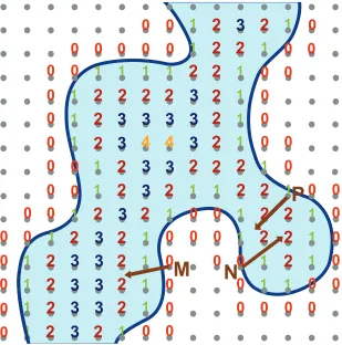
The distance transform maps each image pixel into its smallest distance to a given region of interest (ROI),23_which

can help to distinguish the different structures in the local neighborhood. As shown in Figure 5, the object in cyan is encompassed by a thick curve, ie, the boundary of ROI. After distance transform, the number on each pixel indicates the square of the smallest distance from the pixel to the thick curve. The arrows at pixels M, N, and P point to the directions of their distance mapping-based gradients. Obviously, we can claim that if the gradient directions at any two pixels differ signiﬁ cantly, like those at M and N, these two pixels belong to different structures. However, the opposite argument does not always hold, ie, any two pixels having slightly-varied

gradient directions are not guaranteed to originate from the same structure, like pixels M and P in Figure 5. Wijk and colleagues22_{quantiﬁ ed this by the conﬁ dence value of 0 or 1}

in a diagonal matrix in their normalized convolution method to address the interference between different structures. How-ever, we noticed that the above criterion of differentiating structures can be adaptively incorporated in the widely used convolution method16_{by simply modifying the convolution}

weights as

f x f x angle c x otherwise

1

1 0

0

'

( )=⎧_⎨ ( ) ( , )<

⎩

θ

(2)

where l varies among 0, 1, and 2, and f₁(x) is formulated in Equation 1. f´₁(x) denotes the modiﬁ ed version of f₁(x). Notation angle (c, x) evaluates the angle between the center pixel c and any neighboring pixel x, in terms of the distance mapping-based gradient directions. θ₀ is the predefined thresholding angle, like 90 degrees. Therefore, most pixels in the convolution window but belonging to other structures are excluded from center pixel c in the following convolution operation. However, if the convolution window is too big, some farther pixels will still contribute undesirably to the convolution although they belong to different structures from center pixel c. For example, pixel P will contribute to the convolution operation centered at pixel M, if the distance between pixels P and M is shorter than half of the convolution window size. Fortunately, according to Equation 1, a longer distance from the center pixel will lower down the weights exponentially, and the adverse contributions to the convolution

a) b)

Figure 4 a) A 31 × 31 neighborhood of the red pixel when α1 was set to be 0.719 with truncation value to be 0.00005. b) The zoomed image in the neighbor window of the voxel

at the red cross position indicating the 8 mm polyp in Figure 3. Voxels A and B belong to another structure and they are interfered with the voxel at the red cross position.

(6)

Zhu et al

will be effectively reduced. Therefore, the robustness of such adaptive convolution method can be guaranteed, and its capability of relieving the interference of different structures has been demonstrated by a phantom study.24

In this paper, we refer to the thick curve in Figure 5 as the starting layer (SL) of the distance transform. The overall performance of differentiating different structures in terms of the derived distance ﬁ eld is largely determined by the speciﬁ ed SL. However, the previous work22_{segmented the}

air-tissue interface, serving as the SL, simply by using a thresholding method and ignoring the PVE. While the soft image segmentation algorithm used by Liang and Wang10

was later employed by Wang and colleagues24_{and led}

to a volumetric mucosa to represent the colon wall more accurately, the SL was not properly selected yet, which was just the mucosa-tissue interface as shown in Figure 6b by the red dotted curve. The major problem of this mucosa– tissue interface is its failure to detect the 10 mm polyp due to the severe PVE, along with the remaining interference near the polyp. An alternative layer, ie, the mucosa–air layer, might serve as the SL as well. However such layer, as illustrated in Figure 6b by the blue dotted curve, may

also deform the colon wall in the sense that the concave structure at the neck of the polyp, as blue arrow indicated, has been artiﬁ cially distorted towards an opposite direction. In this paper, we are motivated to introduce a level set-based adaptive convolution (LSAC) method, where a better SL, reﬂ ecting the colon wall more accurately, is generated to improve the adaptive convolution.

Level set framework is one of the geometric deformable models and is based on the curve evolution theory.33_Compared

with other methods, it is able to combine region-based and edge-based information together, make use of global and local information simultaneously and control the geometric property of level set function easily. We intentionally introduce the level set method to retrieve a better SL, from which we build the distance transform to distinguish different topological structures.

Considering the PVE, the SL interface best depicting the shape of colon wall is absolutely not the outermost layer (the mucosa–tissue layer, the red dotted line in Figure 6b) or the innermost layer (the mucosa–air layer, the blue dotted line in Figure 6b) of the VM. Intuitionally, it is located in between the outermost and innermost layers, where

1

0

0 0 0

0

0 0 0

0

0 0 0

0 0 0 0 0

0

0 0 0

0

0 0 0

0

2

0

2

2 2 2

2

3

3 3 3

3

4

3 M

_N

P

Figure 5 The distance transform used to distinguish different topological structures.32

(7)

the variation of CT intensities across the different layers remains relatively stable. Therefore, we extended the C–V model34_{to multi-scale space, where the global and local}

intensity distribution properties are taken into consideration. Speciﬁ cally, the gradient of image intensity is used to con-struct the evolution stopping rule, so that

φ δ φ λ μ

μ

t

in out

B in

I I I I I

I I

= ⋅

+ ∇ ⎡⎣⎢ − − −

⎤ ⎦⎥ ⎧

⎨ ⎩

+ − −

−

( ) ( ) ( )

( )

1 0

2 2

1

2

−

(( )

( ) ( )

I I

I I I I

B out

n in

n out

− ⎡

⎣⎢

⎤ ⎦⎥

+ ⎡ − − −

⎣⎢

⎤ ⎦⎥+

∇ ∇

−

2 2

3

μ μdiv φ

φφ

⎛ ⎝ ⎜⎜ ⎞_⎠⎟⎟⎫⎬⎪

⎭⎪

(3)

where φ is the Lipschitz function, and I represents the image intensities. The two superscripts in and out indicate the regions where φ⬎0 and φⱕ0, respectively, while I,

IB, and In represent the mean intensity values of the whole

image, voxels in the narrow band and the local neighborhood respectively. The notations λ, μ₀, μ₁, μ₂, and μ₃ are controlling

parameters, and ∇ represents the gradient operator.

div ∇

∇ ⎛ ⎝

⎜⎜ ⎞

⎠ ⎟⎟

φ

φ is the curvature of Lipschitz function, which

determines the smoothness of the zero level set surface. Once Equation 3 converges, the resulting zero level set surface of φ= 0 indicates a layer between the outermost and innermost layers, with slightly-changed CT intensities coming across different layers. As described in Figure 6b by the green dotted curve, the acquired zero level set surface

signiﬁ cantly improves the geometric representation of the colon wall.

The middle-layer enhanced integration

(MEI) strategy

After applying the above LSAC strategy and the curvature computation method,16_{geometric measures, like the gradient,}

the ﬁ rst and second principal curvatures, can be retrieved for each voxel in the VM. Similar to our previous work,24_we

further smooth the geometric measures c_i, eg, the principal curvatures, via the following convolution operation

ci _x _LW x c dxi j j j _x _LW x dxi j j

j j

=

_∫

_∈ ( )

_∫

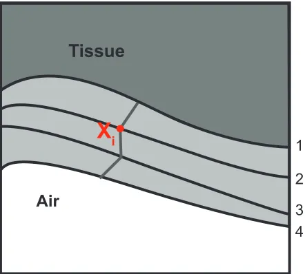
_∈ ( ) (4)

where L is the path starting from the concerned voxel x_i along the positive and negative gradient directions inside the VM, as shown in Figure 7. The Gaussian distributed weight W_i(x_j) was deﬁ ned as W xi( j)=exp(− xj−xi j ) j, xj∈L

2 2

2σ 2πσ

with the standard deviation formulated as σj j

n j r

a b w w

= + ⋅( ⋅ ),

where a and b are predefined constants. The term Wj r

represents the ratio of the local smoothness of x_j to the global one along the path L, whose details are referred

to by Wang and colleagues.24_{However, following the}

same arguments as we acquired SL above, we believe the middle layers (eg, layers 2 and 3 in Figure 7) of the VM would be more reliable than the other layers (eg, layers 1 and 4 in Figure 7) for evaluating the geometric features of the colon mucosa. Therefore, we introduced the MEI

a) b)

Figure 6 a) One slice of a supine image, where the red arrow indicates a 10 mm tubular adenoma. b) The zoomed lumen image near the 10 mm polyp (pointed with the red arrow). The red and blue dotted curves represent the mucosa-tissue and mucosa-air layers respectively, while the green dotted curve is the new SL generated with the level set method in this paper.

Abbreviation: SL,single layer.

(8)

Zhu et al

strategy to highlight the middle layers of the VM through the term Wj

n

Taking Figure 7 as a typical example with totally four layers inside VM and starting from layer 1, the breadth-ﬁ rst dilation strategy marches towards layers 2, 3, and 4. For the presentation simplicity, we simply labeled the dilation step as the layer number when attached to each voxel inside the VM (as shown in Figure 7). Once all the layer numbers are determined, the weight Wj

n

is formulated as:

Wj n n n

n j

= − (5)

where n_j is the layer number of voxel x_j on the path, while

nis the mean value of the layer numbers of all voxels on the path. Voxels with layer numbers close to n are those in the middle of the path, and therefore they have smaller values of Wj

n_{in Equation 5, smaller standard deviations}

j

σ

in the Gaussian model, and ﬁ nally higher weights of W xi( )j in Equation 4.

After applying Equation 4 by means of the MEI strategy, the ﬁ rst and second principal curvatures were reﬁ ned and denoted by k1MEI and

2

MEI

k , respectively, from which the shape index SI (indicates the type of the surface) and curvedness CV

(indicates how curved the surface is) were computed35

1 2 1 2

1 2 2 2

0.5 (1 )arctan( )

( ) ( ) 2

MEI MEI MEI MEI

MEI MEI

SI k k k k

CV k k

π

= − + −

= + (6)

where k1MEI ≠k2MEI. One step further, by reinterpreting the geometric measures c_i in Equation 4 as SI and CV

respectively, the smoothed version, denoted as SI_MEI and

CV_MEI, are acquired to further exploit the correlations between different layers in the VM.

Polyp candidate extraction

As assumed in the previous CAD reports,11–15,25,26_{the upper}

part of the colonic polyps usually appears as a “spherical cap” bulging into the colon lumen. However in our CAD pipeline, the colon lumen image I_L (ie, the percentage distribution map in the range of [0, 1]) views the polyps oppositely. Therefore, the colonic polyps appear as “spherical cups” in the lumen image. Given SI_MEI and CV_MEI as obtained in The middle-layer enhanced integration (MEI) strategy, the variations on the colon wall with local “spherical cup” shapes can be detected by the use of a simple clustering rule.12_However,

the geometric measures, like the shape index and curvedness, are very sensitive to the small variations on the colon wall. Usually, more than one hundred suspicious patches would be generated including a great number of nonpolyp ones. To eliminate the nonpolyp patches as many as we can in this stage, we followed our previous work25_{to remove}

those patches whose sizes were smaller than the clinically-important colonic polyps (eg, larger than or equal to 5 mm in diameter).

Colonic structures, like feces and prominent folds, mimic the spherical shape of true polyps. It’s difﬁ cult to identify the colonic structures from polyps by using only geometric information. To deal with such cases, analyzing the internal textural features for each detection would be an effective way.25_{For the purpose of conducting textural analysis, a}

volume of interest (VOI) is extracted for each suspicious patch. Because of the small contrast, it’s hard to identify the border between a polyp and its surrounding normal tissue. Wang and colleagues25_{assumed that ellipsoid was a choice}

to approximate the shape of polyps. However, the shape of the outer part of polyps bulging into the colon lumen varies greatly, like sessile, pedunculated and ﬂ at shapes. Therefore, the assumption of elliptical region of interest (eROI)25_might

be violated in some cases and consequently include unwanted voxels. Nappi and colleagues26_{introduced an iterative}

conditional morphological dilation method to extract the VOIs. This method proceeded with morphological dilation, which terminated if a minimum growth rate was detected or a predefi ned dilation distance was reached. Advantages of this method lie in the real refl ection of the outer border of polyps. It works fi ne for pedunculated polyps, as the minimum growth rate can often be detected under this circumstance. Otherwise, the morphological dilation process would reserve the morphological characters of the starting suspicious patch,

1

2

3 4

Air

Tissue

X

_i

Figure 7 The integral path across the layers of the volumetric mucosa.

(9)

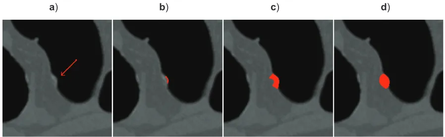
which frequently happens to the sessile and ﬂ at lesions. As shown in Figure 8c, the inner border of the extracted VOI is morphologically similar to the starting region in Figure 8b and still appears as concave, which is generally contradictory to the polyp pathology in general.36_{Therefore, in this study,}

we utilized the inner border generated25_{to stop the dilation}

process when the minimum growth rate cannot be detected. The improved result is shown in Figure 8d.

The grown VOIs are called the IPCs, from which rich textural information can be extracted for the purpose of FP reduction.

FP reduction

For FP reduction, numbers of features were extracted for each IPC to form an associated feature vector. Once we collected all the feature vectors as a sample pool, they were randomly divided into two groups, the training and the testing samples. Given ground truth of the training samples (true positive or false positive, ie, TP or FP), supervised learning machine like LibSVM27_{with nonlinear RBF (radial basis function)}

kernel was trained for maximizing the overall classifi cation accuracy. The classifi er was then applied to the testing samples for prediction. In our study, the sample pool was heavily imbalanced, ie, the number of FPs was signifi cantly larger than that of TPs, such that the cost function was overwhelmed by the contribution of FPs, ie, LibSVM favored the decrease in FPs without ensuring the increase in TPs. Zheng and colleagues37_{reported that the resulting sensitivity was always}

less than 0.5, which was very poor for a CAD scheme. To address the above dilemma, two modiﬁ cations were made based on the LibSVM package:

1. Instead of maximizing the overall classiﬁ cation accuracy, we modiﬁ ed the training goal as minimizing the number

of FP at a speciﬁ ed detection sensitivity of TP, denoted as ζ. By varying ζ (sensitivity levels), we investigated the classiﬁ cation potentials of different feature combinations through fROC (free-response operator characteristics) analysis.

2. Those training samples of TP were assigned larger weights to modulate the imbalanced dataset. In the LibSVM package,27_{the training process was actually a}

procedure of 2D grid search optimizing two parameters to meet the speciﬁ ed goal, ie, the cost function value

C and the RBF kernel parameter γ. We extended such process to a 3D grid search by adding another search for an optimal weight value for TPs. Zheng and colleagues37

assigned a larger value to the parameter C for TPs and a smaller one for FPs to balance the datasets, sharing a similar goal as ours but by a different approach.

In order to evaluate the performance ofLSAC and MEI strategies in CAD applications, we simply employed the four well established geometrical and textual features by Nappi and colleagues,26,38_{which were the mean and variance of}

shape index, the variance of curvedness, and the variance of CT intensity respectively. They were stacked together to form a feature vector for each IPC and fed into the SVM learning package. The output of the SVM would reﬂ ect the gain by the use of the LSAC and MEI strategies.

For the purpose of CAD methodology development, three more aspects would be further considered, in addition to the above presented strategies in steps 1–3 of Figure 1. One is the extraction of more features from the VOI and selection of useful ones for the purpose of detection.39_The

second one is the enhancement of classiﬁ er for improved detection by using the selected features.39_{The third one}

is the presentation of the CAD detection. In what follows,

a) b) c) d)

Figure 8 The VOI extraction for a 6 mm sessile polyp in a sigmoid colon. a) The original polyp (pointed by the red arrow). b) The suspicious patch (the red area). c) The VOI generated with the conditional morphological dilation method.26_d_{) The VOI from our new method.}

Abbreviation: VOI,volume of interest.

(10)

Zhu et al

we give a brief narrative regarding the use of CAD to boost radiologist’s detection performance on polyps everywhere throughout the entire colon.

Detection presentation

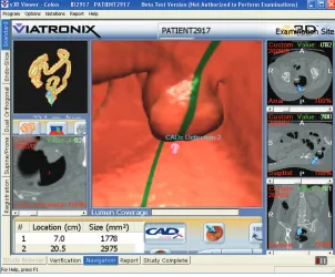
The SVM-reported ﬁ nal polyp candidates are delivered to a commercially available colon visualization system (ie, the V3D-Colon Module; Viatronix Inc, Stony Brook, NY). The system is dedicated to realize the concept of virtual colonoscopy (VC) by mimicking the optical colonoscopy (OC) 3D navigation procedure. Once locating a polyp candidate in such virtual environment, a 3D endoscopic view pops out right in the center screen, along with three cross-sectional views displayed on the right side one after another, as depicted in Figure 9. As a strong supportive module, the CADpolyp pipeline was integrated into the visualization system. Radiologists would then pay more attention to the CAD detected locations and spend less time on other areas of the colon mucosa. In other words, the integrated CAD and visualization system plays the role of computer assisted detection of polyps by human experts.

Performance evaluation

CTC database

To evaluate the performance of the presented CADpolyp pipeline of Figure 1 with the newly developed LSAC and MEI strategies (see the sections on The level set-based adaptive

convolution (LSAC) method and The middle-layer enhanced integration (MEI) strategy, above), VOI extraction (see the section on Polyp candidate extraction, above), and modiﬁ ed SVM parameter setting (see the section on FP reduction, above), twenty-six CTC patient studies, aged from 50 to 80 years old, which were acquired from the University of Wisconsin Hospital and Clinics from July 2006 to April 2007, were used. Each study includes two CT scans, one at supine and the other at prone positions, resulting in 52 CTC datasets. A multi-slice CT scanner (Light Speed Ultra; GE Medical Systems, Milwaukee, WI) was used in helical mode to collect data. The scanning protocol includes modulated mAs in the range of 120–216 mA with kVp of 120–140 values.40_{A total}

of 32 clinically signiﬁ cant polyps were conﬁ rmed with both optical and virtual colonoscopies: nine polyps sized in the range of 5–8 mm and 23 larger than 8 mm with the largest one being 35 mm. In this evaluation, the supine and prone scans of each patient study were considered as different datasets, and the detection sensitivity was evaluated by per polyp and FP rate by dataset (per image). Therefore, there were 64 polyps in 52 CTC images in the CTC database.

Evaluation of initial polyp candidates

(IPC) detection

We set (α₁, α₂) = (1, 0.8) in Equation 1. After applying LSAC method and MEI strategy, those voxels with SI_MEI in [0, 0.06]

Figure 9 Presentation of a polyp candidate, which is a 35 mm sessile polyp in rectum according to the VC and OC reports.

Abbreviations: OC,optical colonoscopy; VC, virtual colonoscopy.

(11)

and CV_MEI in [0.05, 0.14] were labeled as seed, and those in [0, 0.25] and [0.02, 0.5] were identiﬁ ed as growable voxels. Via the above empirically-set thresholds, we could make sure that all the polyps can be initially detected successfully in this stage. Seed voxels were ﬁ rstly clustered together if they were spatially six-connected, grew into suspicious patches by including the six-connected growable voxels. By imposing constraint on the minimal surface area of the found patches, ie, 15 mm2,25_{the surviving suspicious patches penetrated}

into the surrounding tissue area to form IPCs. The locations of the ground truths were determined by physicians, which were represented with the slice numbers in axial, saggital, and coronal directions. These locations were used to specify if a candidate is a TP or FP. If all the 64 polyps were detected successfully and appeared in the resulting group of IPCs, we say that the detection sensitivity in this stage reaches 100% (ie, the by-polyp sensitivity), and the number of false nega-tives (FNs) is zero.

Evaluation of overall performance

of the CADpolyp pipeline

Four features were extracted for each IPC, and stacked together to form a feature vector. The feature vectors of all IPCs were randomly split into two groups of the same size having the same number of TPs, serving as training and testing set respectively. When we conducted the 3D grid search for the optimal parameters C,γ, and ω mentioned in FP reduction, above, the sensitivity level ζ served as the sweeping variable, and varied from 0 to 1. The fi nal perfor-mance was measured based on the testing process. In the testing set, there were 32 true polyps. If all the 32 polyps were classifi ed as TPs, we say that the fi nal detection sensitivity was 100% and there was no FN; while if all the 32 polyps were classifi ed as FPs, the fi nal detection sensitivity would be 0%, and the number of FNs would be maximally 32. However, we could not tell how many datasets there were, since the testing candidates were randomly selected from all the IPCs. In order to calculate the number of FPs per dataset, it’s reasonable to assume that there were 26 datasets in the testing set. As a result, the fi nal performance was presented by using fROC curves.

Results

Performance of IPC detection

Under the pipeline shown in Figure 1, three CAD schemes of detecting IPCs were applied to the CTC image database men-tioned earlier: traditional method, previous or old adaptive method and the presented LSAC method. In the traditional

method (or the fi rst scheme), we just employed the isotropic Gaussian fi lter to compute the fi rst and second derivatives of the images. In the previous adaptive method (or the second scheme), the adaptive method24_{was used. In the third scheme,}

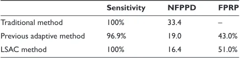
the presented LSAC method was applied. Based on the ﬁ rst and second derivatives of the three schemes, the successive steps with the same parametric conﬁ guration in the pipeline of Figure 1 were applied to extract the IPCs. The IPC extraction performance of these three schemes was shown in Table 1, where the detection sensitivities were evaluated based on datasets. The number of FP per dataset (NFPPD) and the FP reduction percentage (FPRP) based on the traditional scheme were listed in the last two columns.

Compared to the traditional method, the two adaptive schemes signiﬁ cantly reduced the number of FPs (ie, 43% and 51% respectively). However, two polyps, one of which was 10 mm as shown in Figure 6 and the other was a 6 mm tubular adenoma in a prone image, were missed by the pre-vious adaptive method, because the SL used by Wang and colleagues24_{incorrectly depicted the real shape of the colon}

wall near the polyps and failed to recognize the topological structures there. Such problem was rectiﬁ ed by our new LSAC method and even more FPs were reduced.

Performance of overall

CADpolyp pipeline

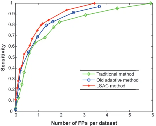
For the three schemes mentioned in the above section, the generated feature vectors of all the IPCs were fed into the same SVM classiﬁ er for the purpose of FP reduction. To evaluate the overall CAD detection performance, three fROC curves in green, blue and red, corresponding to three detection schemes respectively, were generated in Figure 10 as described in the evaluation of overall performance of the CADpolyp pipeline, above, and compared with each other from two different aspects. First of all, the two adaptive methods (red and blue curves) noticeably outperformed the traditional method (green curve). Secondly, the old adap-tive method (blue curve) missed two clinically signiﬁ cant polyps in the stage of IPC detection, and consequently it could not achieve 100% by polyp detection sensitivity. The

Table 1 Performance of the CAD schemes

Sensitivity NFPPD FPRP

Traditional method 100% 33.4 –

Previous adaptive method 96.9% 19.0 43.0%

LSAC method 100% 16.4 51.0%

Abbreviations: CAD, computer-aided detection; FPRP, false positive reduction detection; NFPPD, number of false positives per dataset.

(12)

Zhu et al

presented LSAC method (red curve) solved this problem, and more FPs were reduced. More speciﬁ cally, the traditional method yielded 100% sensitivity with 5.9 FPs/dataset, the previous adaptive method reached 96.9% sensitivity with 3.7 FPs/dataset, and the presented LSAC method achieved 100% sensitivity with 3.5 FPs/dataset.

Discussion and conclusion

In this study, we introduced a LSAC strategy to launch a more meaningful adaptive convolution method, which led to a more accurate geometric analysis on CTC images. Such an improved geometric analysis greatly beneﬁ ted the CADpolyp scheme of Figure 1. In our experiments, the missed polyps in the IPC detection stage by using the previous method24_were

successfully detected with the proposed adaptive convolution strategy, and the number of FPs per dataset was reduced from 19.0 to 16.4, which was a 13.95% reduction. After applying the SVM classiﬁ er, our new CAD scheme yielded 100% sensitivity with 3.5 FPs/dataset.

This paper mainly focused on introducing the LSAC strategy to improve the computation of the ﬁ rst- and second-order derivatives, which was usually the starting point of the geometric analysis. Then, the MEI strategy was applied to exploit the advantage of our volumetric mucosa which was derived from the soft segmentation algorithm.10_The

advantages of the presented CAD scheme (utilizing both LSAC and MEI strategies) were demonstrated with four established features26,38_{together with the well-known SVM}

classiﬁ er. The CAD scheme could be further improved by considering more useful features and using a more powerful classiﬁ er.39

With the above excellent result of 3.5 FPs/dataset at 100% by polyp sensitivity, we noticed that in the ﬁ nal CAD detections, there were still some removable FPs, eg, tubes and ﬂ oating feces. These survived FPs of CAD could be recognized by experts, eg, radiologists, by using a sophisticated visualiza-tion system, eg, the V3D Colon Module system. Therefore, in this paper, we presented an integrated system of CADpolyps and the visualization module which would help the experts further classify the TPs and FPs (see the section on Detection preventation, above). More investigation and validation on the integrated system are under progress.

Inheriting the same assumption regarding the polyps’ spherical-shaped protrusions as the previous CAD schemes did,12,13,25,38_{our CAD pipeline also has lower detection rate,}

as the conventional colonoscopy,12_{for irregularly-structured}

polyps, like those fl at ones. A more generalized model, which is applicable to almost all kinds of clinically signifi cant polyps, deserves our great efforts in the future. The gain of the integrated system for detecting fl at polyps will be another research topic.

We recognize the limitations of our small-sized database with conﬁ rmed and spatially-located polyps. And we are currently devoting ourselves into the access to more datasets. Experienced physicians are invited to locate the (x, y, z) positions of more polyps in our CTC image database. It

0 1 2 3 4 5 6

0 0.1 0.2 0.3 0.4 0.5 0.6 0.7 0.8 0.9 1

Number of FPs per dataset

S

en

s

it

iv

it

y

Traditional method Old adaptive method LSAC method

Figure 10 fROC curves generated by the three schemes. The green, blue and red curves represent the overall detection performances of the traditional, the previous adaptive and the new LSAC method respectively.

Abbreviations: fROC,free-response operator characteristics; LSAC, level set-based adaptive convolution.

(13)

is expected to conduct a more thorough and statistically-signiﬁ cant evaluation of the presented CAPpolyp pipeline.

Acknowledgments

This work was partially supported by NIH Grant #CA082402 and #CA120917 of the National Cancer Institute. The authors would like to acknowledge the use of the Viatronix V3D-Colon Module (or VC visualization and navigation system). The authors would appreciate the comments of Dr Matthew Barish on this work, and the assistance from Dr Hongyu Lu for data processing and Ms Aimee Minton for editing this paper.

References

1. Jemal A, Siegel R, Ward E, Murray T, Xu J, Thun M. Cancer Statistics–2007. CA Cancer J Clin. 2007;57(1):43–66.

2. Eddy D. Screening for coloretal cancer. Ann Intern Med. 1990;113: 373–384.

3. Gluecker T, Johnson C, Harmsen W, et al. Colorectal cancer screening with CT colonography, colonoscopy, and double-contrast barium enema examination: prospective assessment of patient perceptions and preferences. Radiology. 2003;227(2):378–384.

4. Levin B, Brooks D, Smith R, Stone A. Emerging technologies in screening for colorectal cancer: CTC, immunochemical fecal occult blood tests, stool screening using molecular markers. Can J Clin. 2003;53(1):44–55.

5. Pickhardt P, Choi J, Hwang I, et al. Computed tomographic virtual colonoscopy to screen for colorectal neoplasia in asymptomatic adults.

N Engl J Med. 2003;349(23):2191–2200.

6. Bogoni L, Cathier P, Dundar M, et al. Computer-aided detection (CAD) for CT colonography: a tool to address a growing need. Br J Radiol. 2005;78:s57–s62.

7. Taylor SA, Halligan S, Burling D, et al. Computer-assisted reader software versus expert reviewers for polyp detection on CT colonography.

Am J Roentgenol. 2006;86:696–702.

8. Halligan S, Taylor SA, Dehmeshki J, et al. Computer-assisted detection for CT colonography: external validation. Clin Radiol. 2006;61:758–763. 9. Bielen D, Kiss G. Computer-aided detection for CT colonography:

update 2007. Abdom Imaging. 2007;32:571–581.

10. Liang Z, Wang S. An EM approach to MAP solution of segmenting tissue mixtures: a numerical analysis. IEEE Trans Med Imaging. 2009;28(2):297–310.

11. Summers RM, Beaulieu CF, Pusanik LM, et al. Automated polyp detector for CT colonography: feasibility study. Radiology. 2000;216: 284–290. 12. Yoshida H, Nappi J. Three-dimensional computer-aided diagnosis

scheme for detection of colonic polyps. IEEE Trans Med Imaging. 2001;20(12):1261–1274.

13. Nappi J, Frimmel H, Dachman A, Yoshida H. Computerized detection of colorectal masses in CT colonography based on fuzzy merging and wall-thickening analysis. Med Phys. 2004;31(4):860–872.

14. Kiss G, Cleynenbreugel J, Thomeer M, Suetens P, Marchal G. Computer-aided diagnosis in virtual colonography via combination of surface normal and sphere ﬁ tting methods. Eur Radiol. 2002;12:77–81. 15. Paik D, Beaulieu C, Rubin G, et al. Surface normal overlap: a

computer-aided detection algorithm with application to colonic polyps and lung nodules in helical CT. IEEE Trans Med Imaging. 2004;23(6):661–675. 16. Monga O, Benayoun S. Using partial derivatives of 3D images to

extract typical surface features. Comput Vis Image Underst. 1995;61(2): 171–189.

17. Deriche R. Using Canny’s criteria to derive a recursively implemented optimal edge detector. Int J Comput Vis. 1987;1(2):167–187.

18. Thirion JP, Gourdon A. Computing the differential characteristics of isointensity surfaces. Comput Vis Image Underst. 1995;61(2):190–202. 19. Campbell SR, Summers RM. Analysis of kernel method for surface

curvature estimation. Int Congr Ser. 2004;1268:999–1003.

20. Huang A, Summers RM, Hara AK. Surface curvature estimation for automatic colonic polyp detection. Proc SPIE Med Imaging. 2005;5746:393–402.

21. Sundaram P, Zomorodian A, Beaulieu C, Napel S. Colon polyp detection using smoothed shape operators: preliminary results. Med Image Anal. 2008;12:99–119.

22. van Wijk C, Truyen R, Gelder RE, Vliet LJ, Vos FM. On normalized convolution to measure curvature features for automatic polyp detection.

MICCAI. 2004;3216:200–208.

23. Rosenfield A, Pfaltz JL. Sequential operations in digital picture processing. J ACM. 1966;13(4):471–494.

24. Wang S, Zhu H, Lu H, Liang Z. Volume-based feature analysis of mucosa for automatic initial polyp detection in virtual colonoscopy.

Int J Comput Assist Radiol Surg. 2008;3(1–2):131–142.

25. Wang Z, Liang Z, Li L, Li X, Anderson J, Harrington D. Reduction of false positives by internal features for polyp detection in CT-based virtual colonoscopy. Med Phys. 2005;32(12):3602–3616.

26. Nappi J, Yoshida H. Feature-guided analysis for reduction of false positives in CAD of polyps for computed tomographic colonography.

Med Phys. 2003;30(7):1592–1601.

27. Chang CC, Lin CJ. LIBSVM: A library for support vector machines. 2001. [Cited on Jan 10, 2009]. Available from: http://www.csie.ntu. edu.tw/∼cjlin/libsvm.

28. Liang Z, Yang F, Wax M, et al. Inclusion of a priori information in segmentation of colon lumen for 3D virtual colonoscopy”. In:

Conference Record of IEEE Nuclear Science Symposium-Medical Imaging Conference, Albuquerque, NM; 1997.

29. Zhu H, Pickhardt P, Wang S, Posniak E, Cohen H, Liang Z. Computer-aided Detection of Colonic Polyps with a Limited Anisotropic Diffusion in Volumetric Mucosa. The 11th International Conference of MICCAI, Workshop on Computational and Visualization Challenges in the New Era of Virtual Colonoscopy, Sept. 6, New York City. NY; 2008. p. 46–51. 30. Perona P, Malik J. Scale-space and edge detection using anisotropic

dif-fusion. IEEE Trans Pattern Anal Mach Intell. 1990;12(7):629–639. 31. Haberman R. Applied Partial Differential Equations, 4th ed. Upper

Saddle River, NJ: Prentice Hall; 2005.

32. Bitter I, Kaufman AE, Sato M. Penalized-distance volumetric skeleton algorithm. IEEE Trans Vis Comput Graph. 2001;7(3):195–206. 33. Sethian JA. Level Set Methods and Fast Marching Methods: Evolving

interfaces in computational geometry, ﬂ uid mechanics, computer vision, and materials science, 2nd ed. Cambridge: Cambridge University Press; 1999.

34. Vese LA, Chan TF. A multiphase level set framework for image segmentation using the mumford and shah model. Int J Comput Vis. 2002;50(3):271–293.

35. Dorai C, Jain AK. COSMOS-A representation scheme for 3D gree-form objects. IEEE Trans Patt Anal Mach Intel. 1997;19:1115–1130. 36. Haggitt R, Glotzbach R, Soffer E, Wruble L. Prognostic factors in colorectal

carcinomas arising from adenomas: Implications from lesions removed by endoscopic polypectomy. Gastroenterology. 1985;89(1):328–336. 37. Zheng Y, Yang X, Beddoe G. Reduction of false positives in polyp

detection using weighted support vector machines. Conf Proc IEEE Eng Med Biol Soc. 2007;2007:4433–4436.

38. Nappi J, Dachman A, MacEneaney P, Yoshida H. Computer-aided detection of polyps in CT colonography: evaluation of volumetric features in differentiating polyps from false positives. Int Congr Ser. 2001;1230:676–681.

39. Zhao X, Zhu H, Wang S, Liang Z. Reduction of false positives by machine learning for computer-aided detection of colonic polyps. SPIE Med Imaging. 2009; In press.

40. Kim D, Pickhardt P, Taylor A, et al. CT colonography versus colo-noscopy for the detection of advanced neoplasia. N Engl J Med. 2007;357(14):1403–1412.

(14)