Limits of TMD evolution in SIDIS at moderate Q
Leonard Gamberg1,a
1Division of Science, Penn State University Berks, Reading, Pennsylvania 19610, USA
Abstract. We investigate semi-inclusive deep inelastic scattering measurements in the region of relatively smallQ, where sensitivity to nonperturbative transverse momentum dependence can dominate the evolution. Using SIDIS data from the COMPASS experiment, we find that regions of coordinate space that dominate in TMD processes when the hard scale is of the order of only a few GeV are much larger than those commonly probed in largeQmeasurements. This suggests that the details of nonperturbative effects in TMD evolution are especially significant in the region of intermediateQ. We emphasize the strongly universal nature of the nonperturbative component of evolution. and its potential to be tightly constrained by fits from a wide variety of observables that include both large and moderateQ.
1 Introduction
TMD factorization separates a transversely differential cross section into a perturbatively calculable part and sev-eral well-defined universal factors [1], including the trans-verse momentum parton distribution functions fragmen-tation functions. The latter are interpreted in terms of hadronic structure. For example, the TMD factoriza-tion theorems for semi-inclusive deep inelastic scattering (SIDIS) is schematically:
dσSIDIS=
X
f
Hf,SIDIS(αs(µ), µ/Q)⊗Ff/H1(x,k1T;µ, ζ1)
⊗DH2/f(z,k2T;µ, ζ2)+ YSIDIS, (1)
where similar expressions hold for Drell-Yan scattering (DY), and inclusive e+e− annihilation into back-to-back hadrons (e+e− → H1 +H2 + X). The first term is a
generalized product of three factors which closely resem-ble a literal TMD parton model description. The factor,
H(αs(µ), µ/Q) is the hard part, specific to the process, with the other two factors being the universal TMD PDFs and/or FFs, Ff/H1,2 and DH1,2/f (Note, in the case of
“T-odd” TMDs, like the Sivers function [2], universality is predicted to be generalized [3, 4]). The kinematical argu-ments,Q,x1,2andz1,2have standard definitions which can
be found, for example, in Ref. [1]. The TMDs contain a mixture of both perturbative and nonperturbative contribu-tions. But regardless of whether or not they are predomi-nantly described by perturbative or nonperturbative behav-ior, they are universal, and so may be regarded as being as-sociated with individual specific hadrons. TheYSIDISterm
in Eq. (1) provides corrections for the region of large trans-verse momentum of orderQwhere a description in terms of factorized TMD functions is no longer appropriate.
ae-mail: [email protected]
In the QCD evolution of TMDs, the evolution kernel includes both a perturbative short-distance contribution as well as a large-distance nonperturbative, but strongly uni-versal contribution. A unique aspect of TMD evolution is that the kernel for the evolution itself becomes nonpertur-bative in the region of large transverse distances. More-over, one of the important predictions of the TMD factor-ization theorem [1], and a central component to the anal-ysis of TMD evolution, is that the nonperturbative contri-bution to evolution is totally universal, not only with re-spect to different processes, but also with respect to the species of hadrons involved. Furthermore, the soft evolu-tion is independent of whether the TMDs are PDFs or FFs, and is independent of whether the hadrons and/or partons are polarized.1 Therefore, a parametrization of the
non-perturbative evolution from theQdependence in one ob-servable strongly constrains the evolution of many other observables across a wide and diverse variety of different kinds of experiments and for both TMD PDFs and TMD FFs. This strong form of universality is, therefore, an im-portant basic test of the TMD factorization theorem. It is related to the soft factors – the vacuum expectation values of Wilson loops – that are needed in the TMD definitions for consistent factorization with a minimal number of arbi-trary cutoffs. Constraining the nonperturbative component of the evolution probes fundamental aspects of soft QCD.
Semi-inclusive deep inelastic scattering experiments are particularly suited to an examination of the variation in transverse momentum distributions with relatively low
Qand approximately fixedx,zandQ[5]. The COMPASS experiment has released data [6] for charged hadron SIDIS measurements that are differential in all kinematical pa-rameters and cover a range of moderately low values ofQ. We will use this to study theQdependence in the region
1The only dependence is on whether the target partons are quarks or
gluons. C
Owned by the authors, published by EDP Sciences, 2015
of small Qwithin the same experiment and for approxi-mately fixedx,z. The species of hadrons in Ref. [6] is not fixed; the target is6LiD while the measured final state par-ticles include all positively (negatively) charged hadrons. While the range inQin Ref. [6] is too small to allow for reasonably accurate fits to the nonperturbative evolution, it is significant enough that we can use it to rule out any dramatic variations withQthat might be suggested by di-rect didi-rect extrapolations from large Qfits, and to infer certain general aspects of the very large coordinate space
Qdependence [7].
2 TMD Evolution
We summarize the basic formulas of TMD factoriza-tion [1]. The transversely differential cross section for SIDIS in transverse coordinate space, corresponding to Eq. (1), takes the form:
dσ
dP2T ∝ Hf,SIDIS(αs(µ), µ/Q)
Z
d2bTeibT·PT FH˜
1(x,bT;µ, ζ1)
˜
DH2(z,bT;µ, ζ2) + YSIDIS. (2)
We work with the coordinate space integrand in the first term in Eq. (2) and also make the simplifying assumption of quark flavor independence, so we have dropped flavor indices; flavor dependence is easily restored in later for-mulae.2 The kinematical variablesx,zandQfor SIDIS are defined in the usual way, and correspond to those of Ref. [6]. In our notation,Pis the four momentum of the produced hadron,Q2=−q2whereqis the virtual photon momentum,x=Q2/(2PH1·q) wherePH1is the incoming
hadron four-momentum, andz=PH1·P/(PH1·q).PTis the
transverse momentum of the produced hadron in a frame where both the incoming hadron and the virtual photon have zero transverse momentum.
The TMDs in Eqs. (2) contain dependence on the renormalization scale µ and ζ, which are used to parametrize how the effects of soft gluon radiation are par-titioned between the two TMDs [1]. In full QCD, the aux-iliary parameters are exactly arbitrary and this is reflected in the the Collins-Soper (CS) equations for the TMD PDF,
∂ln ˜F(x,bT;µ, ζ1)
∂ln√ζ1
=K˜(bT;µ), (3)
and the renormalization group (RG) equations
dK˜(bT;µ)
dlnµ =−γK(αs(µ)), (4)
dln ˜F(x,bT;µ, ζ1)
dlnµ =γPDF(αs(µ);ζ1/µ
2), (5)
and similarly for the FFs. The anomalous dimensions
γK(αs(µ)) and γF(αs(µ);ζF/µ2) are perturbatively
calcu-lable, and we will keep up to order αs terms. The CS kernel, ˜K(bT;µ), is also perturbatively calculable as long asbT ∼ 1/ΛQCD. Further,ζ1 andζ2 which are not
in-dependent and are related to the physical hard scale Q
2See, however, Ref. [5].
via √ζ1ζ2 = Q2. In full QCD, the auxiliary parameters
are exactly arbitrary, though to optimize the convergence properties of perturbatively calculable parts, a choice of
µ∼ √ζ1 ∼ √
ζ2 ∼Qcan be made. Over short transverse
distance scales, 1/bT is the hard scale, and the transverse coordinate dependence in the TMD PDFs can itself be cal-culated in perturbation theory. With the choice of renor-malization scale µ ∼ 1/bT, αs(∼ 1/bT) approaches zero
for small sizes due to asymptotic freedom ensuring that the small size transverse coordinate dependence is optimally calculable in perturbation theory. For very large bT, the
transverse coordinate dependence corresponds to intrinsic nonperturbative behavior associated with the hadron wave function where a prescription is needed to tame the growth ofαs(1/bT) and match to a nonperturbative, large distance description of the bT-dependence. The renormalization group scale is therefore chosen to be µb ≡ C1/|b∗(bT)|,
whereb∗(b) is a function ofbTthat equalsbT at smallbT,
but freezes in the limit where bT becomes nonperturba-tively large, i.e., whenbT is larger than some fixedbmax.
This function must obey
b∗(bT)=
bT bT bmax
bmax bT bmax.
(6)
The most common taming prescription and the one that we
will adopt here isb∗(bT)≡bT/ q
1+b2
T/b
2
max.The factor
C1 is arbitrary and can be chosen to minimize higher
or-der corrections. It is typically fixed at C1 = 2e−γE. To
put Eq. (2) into a convenient form for perturbative calcu-lations, we express each TMD function evolved from the reference scaleµb. Further since the purpose of this work
is to investigate the largebTbehavior at relatively smallQ,
we define,
gPDF(x,bT;bmax)≡g1(x,bT;bmax) − ln( ˜FH1(x,b∗;µb, µ 2
b))
(7) (and similarly for the FF) where ˜FH1(x,bT;µb, µ2
b) has
op-timal perturbative behavior at smallbT. It is calculable, via an operator product expansion, in terms of collinear PDFs and Wilson coefficients with powers of smallαs(µb) and perturbative coefficients that are well-behaved in the limit ofQΛQCD(and contain no large logs ofbT). Then, we
have for the TMD PDF
˜
FH1(x,bT;Q,Q
2)=exp
(
−gPDF(x,bT;bmax)
−gK(bT;bmax) ln
Q Q0 !
+ln Q
µb
!
˜
K(b∗;µb)
+Z Q
µb
dµ0
µ0 "
γPDF(αs(µ0); 1)−ln
Q µ0 !
γK(αs(µ0))
# )
with a similar expression for the FF. Using these TMDs in Eq. (2) gives the cross section in the compact form:
dσ
dP2T ∝F.T.exp
(
−gPDF(x,bT;bmax)−gFF(z,bT;bmax)
−2gK(bT;bmax) ln
Q Q0 !
+2 ln Q
µb
!
˜
K(b∗;µb)
+Z Q
µb
dµ0
µ0 "
γPDF(αs(µ0); 1)+γFF(αs(µ0); 1)
−2 ln Q
µ0 !
γK(αs(µ0))
#)
+YSIDIS. (9)
The functions gPDF(x,bT;bmax) and gFF(z,bT;bmax)
parametrize the intrinsic large bT behavior associated with the TMD PDF and the TMD fragmentation function respectively. They are independent ofQ. In our notation, they also include, via the definitions Eqs. (7), and the analogous express for the FF [7], the matching to the smallbTbehavior that is calculable using collinear
factor-ization. The functiongK(bT;bmax) on the second line is
the correction to the CS kernel at largebT which includes nonperturbative effects. The underlying simplicity in TMD evolution in that there is a single universal function
˜
K(bT;µ) that governs the evolution of the cross section at smallPT, though in Eq. (9) it has been split into three parts:γK(αs(µ0)), ˜K(b∗;µb), andgK(bT;bmax)3.
With thebT-dependence of the perturbatively calcula-ble part of Eq. (9) frozen above a certainbmax, the
remain-ing evolution is described by the function gK(bT;bmax),
which is totally universal and independent of Q, x, orz.
gK(bT;bmax) generally contains both perturbatively
calcu-lable contributions and nonperturbative effects. By its defi-nition [1], it must vanish like a power at smallbT. Detailed
studies of power corrections in Refs. [8–11] suggest that it vanish likeb2
T(or an even power ofbT) asbT →0.
The value ofbmax, as well as the functional form for the
matchingb∗(bT), is exactly arbitrary in full QCD.
Prac-tically speaking however, dependence on bmax typically
does arise due to incomplete knowledge of the exact form of gK(bT;bmax) at large bT. It is preferable to choose it
to be large enough to maximize the perturbative content of the calculation, while small enough that only a solidly perturbative range ofbT is included in the calculation of
˜
K(b∗;µb). A frequently used ansatz forgK(bT;bmax) is
gK(bT;bmax)=g2(bmax)
1 2b
2
T, (10)
whereg2(bmax) is a Gaussian fit parameter. This choice
forgK(bT;bmax), if positive and reasonably large, imposes
a very strong Gaussian suppression of the nonperturbative regions ofbTin Eq. (9) wheneverQbecomes significantly larger thanQ0. As implied by the notation,g2(bmax) should
be expected to take on different values depending on the choice ofbmax.
3The TMD term in Eq. (9) is derived using the approximation that
PT Q. For an accurate calculation of the full cross section, a
correc-tion term, theY-term, is need for the regionPT∼Q; symbolized by the
last term in Eq. (9). We neglect it, focusing only on the TMD term: a common practice in studies done at moderateQ.
In Ref. [12], parametrizations of the TMD PDFs were constructed out of previous nonperturbative fits within the updated version of the Collins-Soper-Sterman (CSS) for-malism of Ref. [1], and were presented in a form where the contributions to separate operator definitions of the TMD PDFs and fragmentation functions could be automatically identified. These parametrizations were constructed from nonperturbative functions that were extracted in earlier work in the old version of the CSS formalism for DY scat-tering [13, 14], and were combined with fixed scale SIDIS fits at lowQthat arose in the context of hadronic structure studies [15]. A direct extrapolation of the DY fits to low
Qgives evolution that is too rapid [16], and in Ref. [12] this was conjectured to be due to the role of largerxin the small Qfits, so an x-dependent function was inserted to obtain a fit that interpolated between all of the fits, within the TMD evolution formalism.
Recently it was illustrated [16] that the rapid evolu-tion given by extrapolating the nonperturbative extracevolu-tions from DY cross sections at large Qis too fast to account very generally for data in the region of Qof order a few GeV. Thus we have revisited the details of the nonper-turbative contribution to evolution in the region of small
Q[7]. To maintain consistency with the general aim of ex-tracting properties intrinsic to specific hadrons we would ideally varyQwhile holdingx,z, and hadron species fixed. In experiments, however, these variables are correlated, and practical fitting becomes challenging. In the next sec-tion, we use the multi-differential COMPASS data from Ref. [6] to study the variation in the multiplicity distribu-tion with small variadistribu-tions inQand roughly fixed xandz
bins within the same experiment.
3 Empirical Evolution at Moderate
Q
Empirically, the SIDIS data in Ref. [6] reveal that the dif-ferential cross section as a function of PT is reasonably well-described by a Gaussian functional form in the re-gion of small PT (see, e.g., Fig. 4 of Ref. [6]), with a width that broadens very slightly with increasing Q. We have quantified this rate of change within the language of TMD evolution [7]. We then use Eq. (9) to estimate how well it matches the change in widths of the Gaussian fits under different assumptions forgK(bT;bmax).
In Ref. [6], the data for hadron multiplicities are fitted using a Gaussian formdσ/dP2T ∝expn−P2T/hP2Tioand the resultinghP2Tivalues are presented. Expressed in terms of the two dimensional Fourier transform (F.T.) inbT-space,
dσ dP2
T
∝F.T.exp
−b
2
ThP
2
Ti
4
. (11)
Therefore to match to the evolved formula, Eq. (9), we assume that all the terms in the exponent of Eq. (9) can be approximated as quadratic; that is gPDF(x,bT;bmax)
and gFF(z,bT;bmax) ∝ b2T
4. For the moderate Q range
4A note of caution is needed here because the actual behavior of gPDF(x,bT;bmax) andgFF(z,bT;bmax) includes, via the definitions in
of the COMPASS data we consider, where a Gaus-sian fit actually provides a good description of the data, we work with the conjecture that the small bT behav-ior from gPDF(x,bT;bmax) and gFF(z,bT;bmax) is
negligi-ble. However, the details of the initial-scale treatment of
gPDF(x,bT;bmax) andgFF(z,bT;bmax) may become
impor-tant when extending to much largerQ.
A result of CS evolution is that, for the TMD term, the
Q-dependence of the logarithm of the bT-dependence is
linear in ln(Q) [17]. We therefore define,
˜
σTMD term≡ H(αs(Q)) ˜FH1(x,bT;Q,Q
2) ˜DH
2(z,bT;Q,Q
2).
(12) which is the Fourier transform of the TMD term in Eq. (2). Then, CSS evolution of the TMDs gives
dln ˜σTMD term
dlnQ2 b
Tdep
= K˜(bT;µ0)
bTdep , (13)
where the right side is independent ofQ,xandz. Assum-ing that theY-term can be neglected, and using Eq. (11), we then make the approximation that
˜
σTMD term≈exp
−b
2
ThP
2
Ti
4
. (14)
For small PT, the PT-shape of the data in Ref. [6]
is empirically observed to broaden slightly as Q in-creases, but remains quite well described by a Gaus-sian parametrization. Therefore, maintaining the GausGaus-sian shape asQvaries, Eq. (11) must take the form
dσ dP2
T
∝F.T.exp
−b
2
T
4 hP
2
Ti0+4Cevolln
Q2
Q1 !!
. (15)
Here,hP2
Ti0may depend only onxandz(it is independent
ofQ) andCevolis a numerical parameter that is, in
princi-ple, independent ofxandz.Q1andQ2are initial and final
hard scales. If xandzare held fixed, then the variation of hP2
Ti withQcan be found directly from thebT-space
integrand in Eq. (15):
∆hP2Ti(Q1,Q2)≈4Cevolln
Q2
Q1 !
, (16)
where we define∆hP2
Ti(Q1,Q2) =hP
2
TiQ=Q2 − hP 2
TiQ=Q1.
We use Eq. (16) to extract approximate bounds onCevol
from experimental results for∆hP2Ti(Q1,Q2).
The only aspect of TMD factorization that we have used so far is Eq. (13). Specifically, we have applied it to the case of the COMPASS data for the small range of
Q where the PT distribution appears to remain approxi-mately Gaussian even after evolution to obtain Eq. (15). At this stage, we do not address the question of whether
˜
K(bT;µ0) is governed primarily by perturbative or
nonper-turbativebT-dependence. Further, whileCevol resembles
g2 in a quadratic approximation to gK(bT;bmax), here it
should be emphasized that it is meant merely to approx-imate the collective effect of all theQ-dependent terms in
are important for accurately describing the smallbTregion. This
corre-sponds to the behavior of the largePTtail, and accounting for it properly
would involve a careful treatment of theYterm as well.
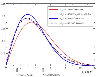
0 2 4 6 8 10 12
bT ( GeV
-1 ) 0
0.05 0.1 0.15 0.2
0.25 0.4 0.8 1.2 1.6 2.0
bT ( fm )
<Q1 2
>=1.10 GeV2
<Q2 2
>= 4.47 GeV2
Initial and Final Gaussian Fits
<Cevol> = 0.0234 GeV 2
Cevol max
= 0.0306 GeV2
Cevol min
= 0.0183 GeV2
<PT
2
>1 = 0.1669 GeV 2
<PT
2 > 2 = 0.2325 GeV
2
0.2< z < 0.25
xbj=0.0295 - 0.0323
» Chiral Scale » Confinement Scale
Figure 1. Coordinate space Gaussian fits showing the largest variation in the
width found in Tables I and II [7] with a change from qhQ2
1i=1.049 GeV to
q hQ2
2i=2.114 GeV. The precise function being plotted is Eq. (17) with the initial
(red) and final (thick blue)hP2
TiCOMPASS values in Eq. (18). The peak moves
to-ward smaller values with increasingQ. We mark the approximate chiral symmetry
breaking scale from Ref. [18] atbT≈1.5 GeV−1and the approximate confinement
scale atbT≈5.0 GeV−1.
the exponent of Eq. (9), in a way consistent with Eq. (13), and it should not be identified at this stage with any spe-cific perturbative or nonperturbative terms. Of course, per-turbative contributions are not quadratic, so the quadratic ansatz for the right side of Eq. (13) is a poor one for small
bT. We nevertheless attempt to use it to capture the general
Q-dependence of thePT-width in the vicinity of smallQ
variations where the data appear from [6] to be reasonably well-described by Gaussian fits. We will further analyze the reliability of such an approximation. Since the right side of Eq. (13) is universal andx,Q, andzindependent, then a test of the universal value forCevolprobes the
as-sumptions that led to the use of Eq. (15) as a model, such as the Gaussian functional form and the neglect of theY -term.
In a full treatment of evolution, there is also aQ de-pendence that affects only the normalization of the cross section. Since we are mainly interested in the variation in the width, we ignore any such contributions and focus only on the broadening of the Gaussian shape.
4
P
T-Broadening & Relevance of Large
b
TEvolution leads to a well-known broadening of the PT
width with Qat fixed xandz. For a significant effect to be clearly observable, one must examine fixedxandzbins over sufficiently broad ranges of Q. In Ref. [6], Figs. 5 and 6 allowQintervals of order∼1.0 GeV for fixedxand
z bins to be identified across several bins in Q. In each panel, the fifth and sixth columns of vertical blocks cor-respond to fixed xandzbins with four and fiveQ2-bins, respectively. Since these give the maximum variation in
Q, they are the data we will use to obtain conservative lim-its on the amount of evolution at moderately small Q. In Ref. [7] we show the results forCevolfrom∆hPT2i(Q1,Q2)
ZQ12^=1.1 GeV2
0.2<z<0.25 xbj=0.0295-0.0323
ZPT2^1=0.1717 GeV2
0.0 0.2 0.4 0.6 0.8 PT
2JGeV2N
0.1 0.2 0.5 1.0 2.0 5.0 10.0 Mulitplicity
Gaussian Fit
ZQ22^=4.47 GeV2
0.2<z<0.25
xbj=0.0295-0.0323
ZPT2^2=0.2477 GeV2
0.0 0.2 0.4 0.6 0.8 1.0 1.2 PT
2JGeV2N
0.2 0.5 1.0 2.0 5.0 Multiplicity
Gaussian Fit
(a) (b)
ZQ12^=1.1 GeV2
0.2<z<0.25
xbj=0.0295-0.0323
ZPT2^
1=0.1717 GeV2
0.0 0.2 0.4 0.6 0.8 PT
2JGeV2N
0 2 4 6 8 10 12 Mulitplicity
Gaussian Fit
ZQ22^=4.47 GeV2
0.2<z<0.25
xbj=0.0295-0.0323
ZPT2^2=0.2477 GeV2
0.0 0.2 0.4 0.6 0.8 1.0 1.2 PT
2JGeV2N
0 2 4 6 8 10 Multiplicity
Gaussian Fit
(c) (d)
Figure 2.(a) Gaussian fit forQ=1.049 GeV, allPT. (b) Gaussian fit forQ=2.114 GeV, allPT. (c, d) Same as (a, b) but on a linear axis. The gray band represents a
99% confidence band for the fit parameters, where only the reported statistical errors have been included.
A limitation of our analysis is the unavoidably largeQ
bin sizes relative toQitself in the moderateQregion. We estimated the error from largeQbin sizes onCevolusing
three methods. We direct the reader to Ref. [7] for details. The trend in Tables I and II and Fig. 2, suggests a small yet non-vanishingQ-dependence in thePTwidth; the
low-est value ofCevolis 0.0040 GeV2 and the largest value is
0.0306 GeV2.
The question of the relevance of the nonperturbative region in the Collins TMD-factorization theorem may be addressed directly in the context of the COMPASS mea-surements by using the fits to estimate the important range ofbT. We have plotted the fits obtained by the COMPASS collaboration [6] in coordinate space as the solid lines in Fig. 1. Since the transverse momentum space distribution is obtained from a two dimensional Fourier transform from the coordinate space expression, we have also included a factor ofbT. Also, since we are primarily interested in the
width of the distribution, we normalize to unity in the in-tegration overbT. Instead of Eq. (14) the curves in Fig. 1 are for
bThP2Ti
2 exp
−b
2
ThP
2
Ti
4
. (17)
Thus, up to a normalization, Eq. (17) is the integrand of the Fourier transform to coordinate space for the region of smallPT.
The initial and final Gaussian slope parametershP2Ti
that we have used in Fig. 1 correspond to thelargest pa-rameterCevolthat is found in Tables I and II [7], yielding
an estimate of themaximumreasonable rate of variation in the width with changes inQof order∼ 1.0 GeV and so is consistent with a strategy of placing rough upper limits on the rate of evolution that can reasonably be expected at
lowQ. The largest value forCevolcorresponds to the
sec-ond row of the first entry in Table II, and the correspsec-onding slope parameters from Ref. [6] are:
hP2TiQ1=1.049 GeV=0.1669±0.0012 GeV2;
hP2TiQ2=2.114 GeV=0.2325±0.0011 GeV
2, (18)
where the uncertainties are the quoted statistical uncertain-ties from the fit only.
The resulting curves shown in Fig. 1 are peaked around
bT ∼ 3.0 GeV−1 with tails extending out to nearlybT ∼
10.0 GeV−1, i.e. up to transverse sizes about twice that of the proton charge radius, suggesting that the effect of nonperturbative input is substantial, at least in this region of moderate Q. From the general features of Fig. 1, we conclude that, for the differential cross section in the limit ofPT →0, the relevant range ofbT is likely to be nearly
dominated by the nonperturbative region of bT for Q ∼
1.0 GeV to∼2.0 GeV.
The robustness of this conclusion might be questioned on the grounds that the fits from [6] apply to a restricted range, PT < 0.85 GeV. One could speculate that includ-ing more of the largePT tail might result in an enhanced relative contribution from small bT. To address this, we have performed our own fit of the Gaussian form using the same data from Ref. [6] that gave the two curves for
Q=1.049 GeV andQ=2.114 GeV in Fig. 1, but now for the entire range ofPT (up toPT &1.0 GeV). We perform the fitting in Wolfram Mathematica. The new Gaussian fits are shown in Fig. 2. From the plot, it is clear that the val-ues we find for the Gaussian slopes,hP2
TiQ1=1.049 GeV and
hP2
TiQ2=2.114 GeV, are so close to the COMPASS values that
in-clusion of largerPT. Instead of Eq. (18), we find:
hP2TiNew FitsQ
1=1.049 GeV=0.1717±0.0011 GeV
2
;
hP2TiNew FitsQ
2=2.114 GeV=0.2477±0.0008 GeV
2, (19)
where again the uncertainties are statistical uncertainties from the fit only. The difference between the COM-PASS fits in Eq. (18) and our fits in Eq. (19) for Q1 =
1.049 GeV is 0.0048 GeV2 and forQ2 =2.114 GeV it is
0.0152 GeV2. This difference gives a sense of the system-atic uncertainty due to the upper cutoffonPT
To see how the new fits affect the coordinate space dis-tribution, Eq. (17), we have replotted in Fig. 3 the original curves from Fig. 1 along with the curves using the new pa-rameters in Eq. (19). It is clear that neglecting the largePT
values has little influence on the general features of the fits discussed above; namely, that there is a large contribution from intervals ofbT deep in the nonperturbative region.
A critique could be made regarding the use of a Gaussian form on the grounds that analyticity consider-ations [19] imply a power law fall-offfor the largePT be-havior of TMD correlation functions. Moreover, a power law behavior 1/P2T (up to logarithmic corrections and the effects of evolution of collinear PDFs) is a prediction of pQCD (see, for example, Ref. [5]). This power law behav-ior is tied to singular behavbehav-ior in the transverse position at smallbT.5 Figure 2(b) shows that the Gaussian form does
have some slight difficulty accounting for the full range of
PT for the largerQ2 =2.114 GeV value. To address this,
we have refitted theQ2 =2.114 GeV data using a Kaplan
functional form:
dσ dP2
T
∝
1+ P
2
T M2
kap −ν
. (20)
The result, shown in Fig. 4, gives a slightly more success-ful fit than the Gaussian fit of Fig. 2(b). When switch-ing from the Gaussian fit to the Kaplan fit it is possible to quantify the goodness of the two fits. We use a straight-forward coefficient of determination,R2, which is defined
in the usual way [20] as 1−SSres/SST, where SSresis the
residual sum of squares of each data point and the fit and SSTis the total sum of squares. This coefficient is a simple
measure of the goodness of the fit that approaches unity for a perfect fit. In this case, theR2fit parameter rises
mod-estly from 0.9918 to 0.9988 when moving from the Gaus-sian form to the Kaplan fit. The final Kaplan fit parameters are Mkap2 =1.3006 GeV2 andν =6.7216. For the lower value ofQ=1.049 GeV, the Gaussian form actually gives a better fit than the Kaplan form. Indeed, from Fig. 2(a) it can be seen that even the Gaussian fit tends to overshoot the data slightly at largePT. This could be due to the role of resonances at very smallQ.
As with the Gaussian form, we may examine the Ka-plan fit in coordinate space. Instead of Eq. (17) we have
2bνTMkap
Γ(ν)
Mkap
2
!ν
K1−ν
bTMkap
, (21)
5The true largeP
T behavior of the TMD functions is not directly
meaningful at very largePT, since TMD factorization (without theY
term) is inapplicable once thePTis comparable withQ. Clearly, theY
-term will be need be incorporated in the future to deal with these issues.
where K1−ν is the order 1−ν modified Bessel function
of the second kind. In coordinate space, the difference
0 2 4 6 8 10 12
b
T ( GeV
-1
)
0 0.05 0.1 0.15 0.2 0.25
<Q1 2
>=1.10 GeV2
COMPASS <Q2
2
>= 4.47 GeV2 COMPASS <Q1
2
>=1.10 GeV2 Our Fit <Q2
2
>=4.47 GeV2 Our Fit
» Chiral Scale » Confinement
Figure 3. Gaussian fits again showing the largest variation in the width found in Tables I and II [7]. The solid red and thick blue curves are the same as those
in Fig. 1, in which the fit is restricted to the region ofPT≤0.85 GeV. The purple
dashed and green dot-dashed curves are from the refit Gaussian curves in Fig. 2 that
use allPTand correspond to Eq. (17)with the initial and finalhP2Tifrom Eq. (19).
between the Gaussian and the Kaplan fits can be examined by comparing Eq. (21) and Eq. (17) with the fit parameters corresponding to Q2 =2.114 GeV. It can be seen that an
analysis of the important regions ofbT leads to roughly the same conclusions as in the case of the Gaussian fit (see Figs. 5 a-d). We conclude that regions ofbT deep into the nonperturbative regime are significant – is robust for
PT → 0 and forQ ∼ 1 GeV to∼ 2 GeV, regardless of which functional form is used.
5 Comparison with TMD Evolution
Next, we examine the evolved formula in Eq. (9) to es-timate how well it matches the change in widths of the Gaussian fits under different assumptions forgK(bT;bmax).
Consider the coordinate space factor in Eq. (9) of the TMD term, including a factor ofbTin analogy with (17):
bT N(Q)exp
(
−gPDF(x,bT;bmax)−gFF(z,bT;bmax)
−2gK(bT;bmax) ln
Q Q0 !
+2 ln Q
µb
!
˜
K(b∗;µb)
+Z Q
µb
dµ0
µ0 "
γPDF(αs(µ0); 1)+γFF(αs(µ0); 1)
−2 ln Q
µ0 !
γK(αs(µ0))
#)
, (22)
whereN(Q) is a normalization factor so that the full quan-tity integrates to unity. We will require that forQ=Q0=
1.049 GeV, Eq. (22) reduces to theQ=1.049 GeV COM-PASS Gaussian fit shown in Fig. 1. which fixes the input functions, −gPDF(x,bT;bmax)−gFF(z,bT;bmax), such that
Eq. (22) reduces exactly to Eq. (17) atQ=Q0[7].
ZQ22^=4.47 GeV2
0.2<z<0.25
xbj=0.0295-0.0323
Mkap2 =1.3006 GeV2
Ν =6.7216
0.0 0.2 0.4 0.6 0.8 1.0 1.2 PT
2JGeV2N
0.2 0.5 1.0 2.0 5.0 Multiplicity
Kaplan Fit
(a)
ZQ22^=4.47 GeV2
0.2<z<0.25
xbj=0.0295-0.0323
Mkap2 =1.3006 GeV2
Ν =6.7216
0.0 0.2 0.4 0.6 0.8 1.0 1.2 PT
2JGeV2N
0 2 4 6 8 10 Multiplicity
Kaplan Fit
(b)
Figure 4. Fits of the Kaplan function, Eq. (20), forQ=2.114 GeV and for
allPT with (a) a logarithmic plot and (b) a linear plot. The gray band represents
a 99% confidence band for the fit parameters, where only the reported statistical errors have been included. (Color online.)
Appendix A of Ref. [7] for reference. We use the approx-imationαs(µ) = 1/2β0ln(µ/ΛQCD) for the running
cou-pling with 3 flavors andΛQCD = 0.2123 GeV Then, the
integrals in the one loop anomalous dimensions may be straightforwardly evaluated to obtain analytic expressions for all perturbative parts of the exponent in Eq. (22) ex-plicit expression is given in App. C of Ref. [7].
For gK(bT;bmax), we start by using Eq. (10), with a
conservativebmax=0.5 GeV−1and several sample values
ofg2(bmax). We compare with the maximum observed rate
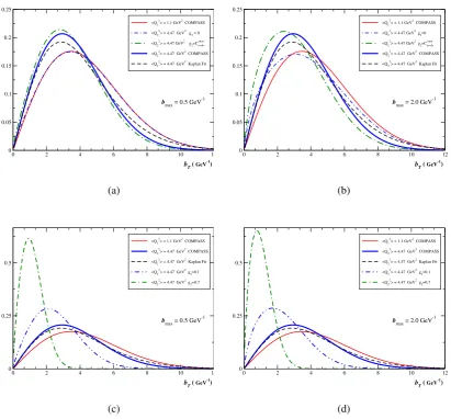
of evolution seen in the COMPASS data – the curves al-ready shown in Fig. 1. The results are shown in Fig. 5(a) and (c), where the dot-dashed curves show the evolution toQ2=4.47 GeV2for a range of sample values forg
2.
We begin with g2 = 0 and see essentially no
ef-fect on the bT distribution when Q is varied; the inte-grand is small in the region of smallbT where perturba-tive evolution would be substantial, and setting g2 = 0
suppresses any nonperturbative contribution to evolution. Next, we considerg2 =Cevol, with the maximum value of
Cevol=0.0306 GeV2. Finally, we considerg2=0.1 GeV2
andg2 =0.7 GeV2 which are values more typical of fits
obtained at large Q, as well as the renormalon analysis value ofg2 =0.19 GeV2in Ref. [9]. (See, also, Fig. 1 of
Ref. [14].)
We repeat this exercise for the much more liberal value of bmax = 2.0 GeV−1, and the result is shown in Figs. 5
(b) and (d). In Figs. 5(a)-(d), a value ofg2(bmax).Cevolmax
is clearly preferred over values ofg2(bmax) ≥ 0.1 GeV2.
Note that withg2 =0, there is very weak evolution in the
bT shape relative to the variations in the width suggested
by the COMPASS data in the small range ofQvalues. A
choice ofg2 =Cmaxevol=0.0306 GeV2is roughly consistent
with the upper limit on the rate of evolution observed in Tables I and II of Ref. [7]. Thus, if we demand the ansatz in Eq. (10) for the form ofgK(bT;bmax) for allbT, then we
estimate that the true value ofg2, must lie roughly in the
range of 0< g2.0.03 GeV2.
6 Modified Large
b
TBehavior
Because of the strong universality ofgK(bT;bmax), the
re-sults of the last section seem on the surface to indicate a discrepancy between the lowQdata and successful fits of the past that focus on larger Q, which tend to findg2 &
0.1 GeV2[13, 14, 21, 22]. For instance, values ofg
2have
been found to be as large as 0.68 GeV2[13], and a value
of g2 =0.19 GeV2 is used in Ref. [22] for SIDIS in the
CSS formalism, both using a value ofbmax =0.5 GeV−1.
However, the quadratic ansatz in Eq. (10) seems to impose excessive suppression of the very large nonperturbativebT
region wheneverg2&0.1 GeV2.
To resolve the apparent discrepancy discussed above, we recall that largeQfits, e.g. forQ&10 GeV, are sen-sitive mainly to the region ofbT . 2.0 GeV−1. See, for
example, Fig. 4 of Ref. [14] and compare this with Fig. 1, where contributions frombT &2.0 GeV−1dominate. Now
let us assume that nonperturbative effects become totally dominant at some large size scalebNP, wheregK(bT;bmax)
acquires a more complicated and as-yet unknown precise form. Recall also thatgK(bT;bmax) is predicted to vanish
as a power ofb2
T at smallbT [8–11]. Thus, forbT bNP
the following expansion applies:
gK(bT;bmax)=a1
b2
T b2
NP
+a2
b4
T b4
NP
+· · ·. (23)
We conjecture that largeQfits typically obtain a largeg2
because they are sensitive only to the first power-law cor-rection in Eq. (23). By contrast, at smallerQhigher pow-ers, and eventually the complete functional form, become important.
We propose that the optimal way to proceed is to use a functional form forgK(bT;bmax) that: a) respects its strong
universality set forth in TMD factorization by matching to earlier largeQfits that use a Gaussian form but b) avoids strong disagreement with the results of the empirical anal-ysis of SIDIS data from Sect. 4. Thus, we impose the fol-lowing conditions: (i) At smallb2
T, the lowest order coeffi
-cient in Eq. (23), i.e.a1/b2NP, must be roughly&0.1 GeV2
in order to be consistent with the values ofg2/2 found in
Ref. [9, 13, 14, 21, 22], thereby respecting the strong uni-versality ofgK(bT;bmax). (ii) AtbT bNP,gK(bT;bmax)
should become nearly constant, or at most logarithmic in
bT. As a simple example, we propose [7]
gK(bT;bmax)=
g2(bmax)b2NP
2 ln
1+
b2
T b2
NP
. (24)
Expanding aroundbTbNPgives the first two terms,
g2(bmax)
1 2b
2
T −g2(bmax)
1 4b2NPb
4
0 2 4 6 8 10 12
bT ( GeV-1)
0 0.05 0.1 0.15 0.2 0.25
<Q 1
2> = 1.1 GeV2 COMPASS
<Q 2
2> = 4.47 GeV2 g 2 = 0
<Q 2
2> = 4.47 GeV2 g 2=Cevolv
max
<Q2 2
> = 4.47 GeV2 COMPASS
<Q2 2
> = 4.47 GeV2 Kaplan Fit
bmax = 0.5 GeV-1
0 2 4 6 8 10 12
bT ( GeV-1)
0 0.05 0.1 0.15 0.2 0.25
<Q 1
2> = 1.1 GeV2 COMPASS
<Q 2
2> = 4.47 GeV2 g 2=0
<Q 2
2> = 4.47 GeV2 g 2=Cevolv
max
<Q2 2
> = 4.47 GeV2 COMPASS
<Q2 2
> = 4.47 GeV2 Kaplan Fit
bmax = 2.0 GeV-1
(a) (b)
0 2 4 6 8 10 12
b T ( GeV
-1 )
0 0.25 0.5
<Q
1
2> = 1.1 GeV2 COMPASS
<Q
2
2> = 4.47 GeV2 COMPASS
<Q
2
2> = 4.47 GeV2 Kaplan Fit
<Q
2 2> = 4.47 GeV2 g
2=0.1
<Q
2 2> = 4.47 GeV2 g
2=0.7
bmax = 0.5 GeV-1
0 2 4 6 8 10 12
b T ( GeV
-1 )
0 0.25 0.5
<Q
1
2> = 1.1 GeV2 COMPASS
<Q
2
2> = 4.47 GeV2 COMPASS
<Q
2
2> = 4.47 GeV2 Kaplan Fit
<Q
2 2> = 4.47 GeV2 g
2=0.1
<Q
2 2> = 4.47 GeV2 g
2=0.7
bmax = 2.0 GeV-1
(c) (d)
Figure 5. Left Panels (a) and (c): The solid red and thick blue lines are the same initial and final Gaussian fits obtained by COMPASS as in Fig. 1 forQ2
1=1.1 GeV
2
andQ2
2=4.47 GeV2respectively. The black dashed curve is the Kaplan fit forQ2=4.47 GeV2, shown in [7]. The dot-dashed lines are the TMD factorization expression
in Eq. (22) for the evolution toQ2
2=4.47 GeV2with the Gaussian ansatz from Eq. (10) forgK(bT;bmax) withbmax=0.5 GeV−1. The positions of the peaks of the evolved
distributions decrease with increasingg2: Figure (a) shows the results forg2=0 (blue dot-dashed) andCmaxevol=0.0306 GeV2(green dot-dashed); Figure (c) shows the result
forg2=0.1 GeV2(blue dot-dashed) andg2=0.7 GeV2(green dot-dashed). All curves are normalized to one in the integration overbT. Right Panels (b) and (d): Same as
the left panels, but forbmax=2.0 GeV−1.
In Fig. 6 we illustrate how the lowQdependence of the COMPASS data may be accommodated into earlier larger
Q fits by using the modified gK(bT;bmax) from Eq. (24)
with bmax = 0.5 GeV−1, g2 = 0.1 GeV2 and bNP =
2.0 GeV−1. Since the lowest order term in the expan-sion in Eq. (25) matches Eq. (10) withg2 =O(0.1 GeV2)
and thus is generally consistent with earlier fits such as Ref. [21, 22]. In this way, moderate Qdata may be ac-commodated without introducing disagreement with im-portant and universal nonperturbative contributions ob-tained in earlier fits, while simultaneously giving access to further universal nonperturbative information. For now we propose Eq. (24) only as a simple example of how
gK(bT;bmax) might possibly be modified at very largebT.
In practice, better and more detailed parametrizations may be needed, possibly obtainable from nonperturbative stud-ies (see e.g. [23]).
By allowing a more general treatment of the non-perturbative component of the CS kernel than the usual power law, we find that we may extend TMD factorization to lowerQSIDIS measurements with no need to distort the perturbative part of evolution that is necessary to unify low
0 2 4 6 8 10 12
bT ( GeV-1)
0 0.05 0.1 0.15 0.2 0.25
<Q 1
2> = 1.1 GeV2 COMPASS
<Q2 2
> = 4.47 GeV2 g2=0.1 bNP=2.0 GeV -1
<Q2 2
> = 4.47 GeV2 COMPASS <Q2
2
> = 4.47 GeV2 Kaplan Fit
» Confinement
» Chiral Scale
Figure 6.The solid red and thick blue curves are again the same initial and final
Gaussian fits obtained by COMPASS forQ2=1.1 GeV2andQ2=4.47 GeV2
respectively – the same as in Fig. 1 . The black dot-dashed curve is the Kaplan
fit forQ2 =4.47 GeV2. For comparison, the purple short-dashed curve is the
TMD factorization expression in Eq. (22), but now using Eq. (24) forgK(bT;bmax=
0.5 GeV−1) withb
NP=2.0 GeV−1andg2=0.1 GeV2. This should be compared
with theg2≥0.1 GeV2curves in Fig. 5 where the quadratic ansatz forgK(bT;bmax),
Eq. (10) is used.
with the much larger nonperturbative soft evolution found from direct extrapolations of global fits of Drell-Yan or largeQprocesses to much lowerQ, if one limits the treat-ment of the nonperturbative largebT evolution factor to the quadratic form in Eq. (10) for allbT. In this regard, we confirm one of the main observations of Ref. [16]. The meaning that we extract from these observations however is very different. In our analysis, we find much greater sensitivity to the details of the nonperturbative large bT
structure, rather than evidence that nonperturbative con-tributions to evolution are unnecessary. By contrast, it has been suggested in Refs. [16, 24], within the context of sim-ilar but alternative evolution formalisms, that accounting for nonperturbative evolution can be avoided entirely even at scales of orderQ∼1.0 to 2.0 GeV. Moreover, we find that the complications that arise from extrapolating from large to moderateQarise because of the greater care nec-essary in treating the nonperturbative contribution to evo-lution as largerbTvalues become relevant to evolution, not because such non-perturbative effects are less relevant (see also and [25]). By accounting for the nonperturbative be-havior at very largebT, as discussed here, we find that it is not difficult to reconcile past largeQfits of nonperturba-tive evolution with the moderateQfits as is displayed in Fig. 6.
Acknowledgements
I thank my collaborators, Christine Aidala, Bryan Field, and Ted Rogers for their work on this project. Discussions with Miguel Echevarria, Ahmed Idilbi, Ignazio Scimemi, and Andrea Sig-nori are gratefully acknowledged. This work is supported by
the U.S. Department of Energy, under contract No. DE-FG02-07ER41460.
References
[1] J.C. Collins, Foundations of Perturbative QCD
(Cambridge University Press, Cambridge, 2011) [2] D.W. Sivers, Phys. Rev.D41, 83 (1990)
[3] J.C. Collins, Phys. Lett. B536, 43 (2002),
hep-ph/0204004
[4] S.J. Brodsky, D.S. Hwang, I. Schmidt, Nucl. Phys.
B642, 344 (2002),hep-ph/0206259
[5] A. Bacchetta, D. Boer, M. Diehl, P.J. Mulders, JHEP
08, 023 (2008),0803.0227
[6] C. Adolph et al. (COMPASS), Eur.Phys.J.C73, 2531 (2013),1305.7317
[7] C. Aidala, B. Field, L. Gamberg, T. Rogers, Phys.Rev.D89, 094002 (2014),1401.2654
[8] G.P. Korchemsky, G.F. Sterman, Nucl.Phys. B437, 415 (1995),hep-ph/9411211
[9] S. Tafat, JHEP0105, 004 (2001),hep-ph/0102237
[10] E. Laenen, G.F. Sterman, W. Vogelsang, Phys.Rev.
D63, 114018 (2001),hep-ph/0010080
[11] E. Laenen, G.F. Sterman, W. Vogelsang, pp. 1411– 1413 (2000),hep-ph/0010183
[12] S.M. Aybat, T.C. Rogers, Phys. Rev. D83, 114042 (2011),1101.5057
[13] F. Landry, R. Brock, P.M. Nadolsky, C.P. Yuan, Phys. Rev.D67, 073016 (2003),hep-ph/0212159
[14] A.V. Konychev, P.M. Nadolsky, Phys.Lett.B633, 710 (2006),hep-ph/0506225
[15] P. Schweitzer, T. Teckentrup, A. Metz, Phys.Rev.
D81, 094019 (2010),1003.2190
[16] P. Sun, F. Yuan, Phys.Rev. D88, 114012 (2013),
1308.5003
[17] J.C. Collins, D.E. Soper, G.F. Sterman, Nucl.Phys.
B250, 199 (1985)
[18] P. Schweitzer, M. Strikman, C. Weiss, Acta Phys.Polon.Supp.6, 109 (2013),1212.4031
[19] P. Schweitzer, M. Strikman, C. Weiss, JHEP1301, 163 (2013),1210.1267
[20] R.E. Walpole, R.H. Myers, S.L. Myers, K.E. Ye,
Probability and Statistics for Engineers and Scien-tists (9th Edition), 9th (Pearson, January 6, 2011) [21] P.M. Nadolsky, D. Stump, C. Yuan, Phys.Rev.D61,
014003 (2000),hep-ph/9906280
[22] P.M. Nadolsky, D. Stump, C. Yuan, Phys.Rev.D64, 114011 (2001),hep-ph/0012261
[23] J. Collins (2014),1409.5408
[24] M.G. Echevarria, A. Idilbi, A. Schafer, I. Scimemi, Eur.Phys.J.C73, 2636 (2013),1208.1281
![Figure 1. Coordinate space Gaussian fits showing the largest variation in thewidth found in Tables I and II [7] with a change from�⟨Q21⟩ = 1.049 GeV to�⟨Q22⟩ = 2.114 GeV](https://thumb-us.123doks.com/thumbv2/123dok_us/8184801.1366880/4.595.322.513.86.238/figure-coordinate-gaussian-showing-largest-variation-thewidth-tables.webp)

![Figure 3. Gaussian fits again showing the largest variation in the width foundin Tables I and II [7]](https://thumb-us.123doks.com/thumbv2/123dok_us/8184801.1366880/6.595.313.539.569.680/figure-gaussian-ts-showing-largest-variation-foundin-tables.webp)