Article
1
A cooperation of multileader fruit fly and the
2
probabilistic random walk with adaptive
3
normalization for solving solution of the
4
unconstrained optimization problems
5
Wirote Apinantanakon 1, Khamron Sunat 2,* and Sirapat Chiewchanwattana 2
6
1 Department of Computer Science, Faculty of Science, Khon Kaen University, Thailand 40002;
7
8
2 Department of Computer Science, Faculty of Science, Khon Kaen University, Thailand 40002;
9
10
* Correspondence: [email protected]; Tel.: +66-80-461-3391
11
12
Abstract: A swarm based nature-inspired optimization algorithm namely fruit fly optimization
13
algorithm (FOA) has simple structure and ease of implementation. However, FOA has a low
14
success rate and a slow convergence because FOA generates new positions around the best location
15
using fixed search radius. Several improved FOAs have been proposed. But their exploration
16
ability is questionable. To make the search process to transit from the exploration phase to the
17
exploitation phase smoothly, this paper proposes a new FOA constructed from a cooperation of the
18
multileader and the probabilistic random walk strategies (CPFOA). It has two population types
19
working together. CPFOA's performance is evaluated by 18 well-known standard benchmark, and
20
30 CEC’2017 functions. The results showed that CPFOA outperforms both the original FOA and its
21
variants in terms of convergence speed and performance accuracy. The results base on CEC’2017
22
show that CPFOA can achieve a very promising accuracy when compared with the well-known
23
competitive algorithms. CPFOA is applied to optimize two applications; the MLPs classifying real
24
datasets and extracting parameters of T-S fuzzy system for modelling Box and Jenkins gas furnace
25
data set. CPFOA can find parameters having a very high quality compared with the best known
26
competitive algorithms.
27
Keywords: nature-inspired optimization algorithm; fruit fly optimization algorithm; multileader
28
strategy; random walk; cooperative algorithm
29
30
31
32
33
34
35
36
37
38
1. Introduction
39
Over the last few decades, researchers have started adapting knowledge from natural
40
phenomena for the development of optimization techniques. The main concepts of the aptly named
41
sources 'nature-inspired algorithms' have been observed within successful biological systems.
42
Accordingly, most nature-inspired algorithms are biologically inspired, or bio-inspired, and mimic
43
specific behavior in nature. Examples of such popular nature-inspired algorithms include the
44
particle swarm optimization algorithm (PSO) [1], which was inspired by the social behavior of
45
flocking birds, or schooling fish; the ant colony optimization algorithm (ACO) [2], which mimics an
46
ant colony's behavior in their search for food; the artificial bee colony algorithm (ABC) [3], motivated
47
by the intelligent behavior of a honey bee swarm; the cuckoo search algorithm (CS) [4], inspired by
48
the parasitic bio-interactions of a cuckoo species that lays their eggs in the nests of other host birds;
49
and the bat-inspired algorithm (BA) [5], which was inspired by the echolocation behavior of bats, to
50
name but a few. However, each nature-inspired algorithm has different capabilities when it comes to
51
finding solutions, which depend on the personal ability of the living things in nature. Developing a
52
successful, modern nature-inspired algorithm is a challenging task, even today, as there is no one
53
particular nature-inspired algorithm capable of solving every scientific problem. Hence the
54
continual development of a new algorithm is required. As can be seen the details and the broadly
55
classified the nature-inspired algorithms, which presented the development of algorithms into the
56
current modern literatures [6,7].
57
In 2011, a swarm intelligence method-based stochastic optimization technique namely the fruit
58
fly optimization algorithm (FOA) was proposed by Pan [8]. It is based upon the foraging behavior of
59
fruit flies. FOA is very user-friendly because of its simplicity and shortness. FOA can be easily
60
understood by most researchers in this field. This also means that it can be easily implemented into
61
program code, when compared with other well-known algorithms such as differential evolution
62
(DE) [9], genetic algorithm (GA) [10] and particle swarm optimization (PSO). The FOA has achieved
63
success in several applications; including research into optimization problems [11-14], neural
64
network parameters optimization [15-17], swarm techniques for mini autonomous surface vehicles
65
(ASVs) [18], identification of dynamic protein complexes based on fruit fly optimization algorithm
66
[19], support vector regression with fruit fly optimization algorithm for seasonal electricity
67
consumption forecasting [20], efficient truss optimization using the contrast-based fruit fly
68
optimization algorithm [21] and improved fruit fly optimization algorithm for application to
69
structural engineering design optimization problems [22,23], a prediction model for China
70
agricultural output value based on the optimization of neural network [24], and a novel phase
71
angle-encoded fruit fly optimization algorithm with mutation adaptation mechanism applied to
72
UAV path planning [25].
73
Pan’s FOA has a good structure and mechanism for the solution finding of optimization
74
problems. However, the algorithm is prone to trapping into a local extreme and premature
75
convergence, since FOA generates new fruit flies swarm around the current best solution by using
76
random uniform distribution with a fixed radius. Especially when FOA deals with
77
multi-dimensional and complex optimization problems.
78
The drawback caused by the fixed radius updating has encouraged many researches effort into
79
various dynamic radius updating techniques to improve the FOA, e.g., an improved fruit fly
80
optimization algorithm for solving optimization problems (LGMS-FOA) [11], an improved fruit fly
81
optimization algorithm for continuous function optimization problems (IFFO) [12], a novel
82
multi-swarm fruit fly optimization algorithm (MFOA) [14], a novel multi-scale cooperative mutation
83
fruit fly optimization algorithm (MSFOA) [26], and a novel fruit fly optimization algorithm with
84
trend search and co-evolution (CEFOA) [27].
85
There is one remaining imperfection that is caused by the single leader usage, although the
86
FOA variants showed that the dynamic radius updating can improve the quality of the produced
87
solutions. The single leader usage makes FOA to lack of diversity when the search process has to
88
deal with a multi-dimensional or a complex optimization problem. In this paper, we proposed a
89
updating instead of random uniform dynamic radius updating (CPFOA). The details of proposed
91
CPFOA are described as in section 3.
92
The remaining of the paper are as follows: Section 2 presents the FOA; Section 3 presents the
93
strategies for CPFOA construction, the multileader, and the probabilistic random walk strategies;
94
Section 4 explains the evaluation process of algorithms and settings; Section 5 shows the
95
experimental results and discussion; Section 6 shows two applications of CPFOA; and lastly, Section
96
7 concludes the paper.
97
2. The Fruit Fly Optimization Algorithm
98
The drosophila optimized algorithm or fruit fly optimization algorithm (FOA) was developed
99
in 2011 by Pan [8]. FOA determines global optimization based on the foraging behavior of fruit flies.
100
Compared to other species, the fruit fly possesses a keener sense of smell and sight in the search for
101
their food. Their drosophila olfactory organ can detect a food source as far as 40 kilometers away,
102
which triggers a flight reaction toward the target location. For the intelligent sense of fruit flies, the
103
novel FOA optimization algorithm is inspired and established through the simple behavior of fruit
104
flies’ search for food.
105
The FOA’s process is similar to as with the other swarm optimization algorithms. The first
106
phase of the fruit flies’ quest for food is initiated with a random uniform distribution [6,28-32], with
107
no specific position or direction. In the second phase, the fruit fly with the best sense of smell or the
108
best fitness from the first phase within the group is determined. The fruit fly with the best sense of
109
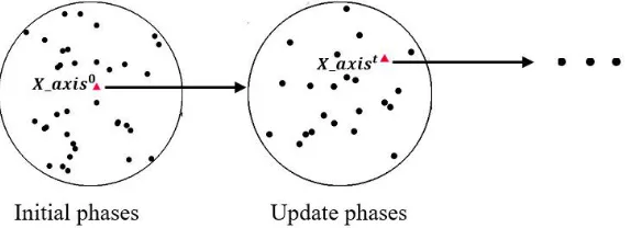
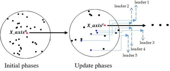
smell is used to be a center for generating the new populations in the next generation. Figure 1
110
illustrates the pattern of the fruit flies’ search for food. Figure 1 (Initial phase), _ is the fruit
111
fly with the best sense of smell that is determined in current generation. In the latter generation, the
112
_ is used to be the center for generating a new position of each individual fruit fly. The
113
computational steps of FOA method are summarized in Algorithm 1.
114
Figure 1. The simulation state of the FOA’s single leader.
115
116
117
118
119
120
121
122
Algorithm 1. The FOA algorithm
Step 1. Initialize FOA’s parameters: random location( _ , _ ), size of population( ),
and the maximum iteration( _ ).
Step 2. Give the random position and fly direction of an individual fruit fly in their search for food.
= _ + ( )
= _ + ( )
Step 3. Calculate the distance ( ) to the food’s origin, as the exact position of the food’s location is
not known at this stage.
= +
Step 4. Calculate the smell concentration judgment value ( ).
=
Step 5. Calculate the fitness: the smell concentration judgment of the individual fruit fly, obtained
from Step 4, is calculated by substituting Si into the smell concentration judgment function (also
called fitness function), in order to find the optimal smell.
Smelli = objective function ( )
Step 6. Determine the fruit fly with the optimal smell concentration judgment among the fruit fly
group.
[bestSmell, bestIndex] = find_the_best (Smell)
Step 7. Keep the best (x, y) position and the optimal concentration value; and use this position as the
center of flying towards the next location (in step 2).
Smellbest = bestSmell
_ = (bestIndex)
_ = (bestIndex)
Step 8. Repeat steps 2-7 and determine whether the smell concentration is better than the previous
iterative smell concentration. If yes, go to step 7. The process will stop if either the smell
concentration no longer changes or the iterative number reaches the maximum iteration
number( _ ). The output are _ and _ .
124
2.1. An Analysis of the Original FOA and the FOA Variants
125
2.1.1. Analysis of the Original FOA
126
There are problems of FOA that makes the algorithm unsuitable to deal with multi-dimensional
127
and complex optimization problems. The problems are investigated in [11,12,14,26,27,33,34] and are
128
briefly described as follows.
129
1. Problems regarding the smell value , in according to Step 4, cannot appropriately evaluate
130
the “objective function ( )” when there are negative numbers in the domain because
131
= / > so that the function cannot determine as negative [11,14,33,34]
.
132
2. The fixing radius with random uniform distribution within the initial process limited the
133
2.1.2 Analysis of the FOA Variants
135
To overcome the disadvantages of the original FOA, researchers have developed continuously
136
new strategies to improve the FOA for solving high-dimensional function optimization problems.
137
The recently proposed FOAs can be found in the two categories. The first category is defining each of
138
fruit flies through the random initial base point of _ , _ and the positions of and
139
as in the original FOA for updating the new generation of populations. The other functions, such as
140
smell value ( ) and the evaluating of the objective function ( ), are modified with including the
141
extra mechanisms. The second category is trying to solve these the problems by (i) omitting , (ii)
142
defining each of fruit flies through ∈ ℝ × , where D is the number of decision variables (or
143
dimensions), and N is the population size, i.e., = , , , … , ∈ ℝ , and (iii) removing the
144
distance and smell concentration judgment function . The fitness value is now calculated
145
by substituting into the smell concentration judgment function with Smelli = objective_function
146
( ). The position of the fruit fly having the minimal concentration value, _ , is the base point
147
for flying towards the next location. A brief summary of the two categories improved FOAs are as
148
follows.
149
The first category is as follow.
150
Babalık et al. [35] proposed an improvement in fruit fly optimization algorithm by using sign
151
parameters (SFOA). The algorithm presents the improvement method by using two sign
152
variables r and q vectors in order to determine a sign for each decision variable of fruit flies.
153
CEFOA [27] proposed by Han et al. revealed that the simple structure of FOA limited the search
154
space and made the fruit flies to be trapped into a local minimum easily. To overcome the
155
drawback, the CEFOA used two mechanisms; the trend search strategy and the co-evolution
156
mechanism. The trend search enhances the local search capability of swarm. The co-evolution
157
mechanism is employed to avoid the premature convergence and to improve the global
158
searching ability. However, the key of the CEFOA is the multi-scales equation for updating fruit
159
fly swarm. To set the variable capacity of each fruit fly connecting with its food quality, the
160
CEFOA used the variance of the multi-level evolutionary operator. The search radius is
161
dynamically adjusted through ( ) = ( − ) + × ( , ( )) and ( ) = ( − ) +
162
× , ( ) , where ( ) are the multi-scale factor of i-th fruit fly.
163
The second category is as follow.
164
LGMS-FOA, proposed by Shan et al. [11], presented two parameters to tune up the search
165
radius by adding the weight parameter w when the radius is changed with respect to time. A
166
new fruit fly location is generated as = _ + × [ , ), = × , where
167
= , = . , t = iteration index, and _ is the best position obtained during
168
iterations.
169
IFFO, proposed by Pan et al. [12], introduced a new control parameter to adjust the search
170
radius adaptively. The search radius is dynamically changed during iterations through =
171
× ( ( / ) × / ), where is the radius variants in each iteration, =
172
( − )/ , is the upper bound and is the lower bound of domain problems,
173
= , is the iteration index and is the maximum iteration number ( _ ).
174
MFOA, proposed by Yuan et al. [14], presented a multi-swarm fruit fly that employed
175
sub-swarm to explore the solutions in the search space simultaneously. Moreover, MFOA
176
shrinks the search radius through ( ) = ( − / ) × ( − / ) , where t is the
177
iteration index, is the upper bound, is the lower bound, is the number of
178
sub-swarms and is the maximum number of sub-swarms.
179
MSFOA, proposed by Zhang et al. [26], presented a strategy to analyze the convergence and
180
showed that the convergence depends on the initial positions of swarms. MSFOA used the
181
details in [26]). For a fruit fly flying, MSFOA used a linear generation mechanism, through the
183
equation of , = + × ( , ), where = × , = , = . , is
184
current iteration, is the search coefficient, is the initial weight and , are
185
obtained from the domain boundary of the problem.
186
To recap, the improved FOAs such as SFOA, CEFOA, LGMS-FOA, IFFO, MFOA and MSFOA
187
were proposed strategies to enhance the search ability. The search radius was a main tackle point in
188
several proposed. However, only the dynamical mechanism of the search radius itself might not
189
enough efficient for overwhelming the lacking of diversity and premature convergence because
190
these FOA variants still used only one leader as the flying base point. The single leader strategy
191
might affect to FOA in to be trapped in a local optimum easily when to optimize a multi-dimensional
192
optimization problem. In this paper, the proposed CPFOA comprises of two strategies. The first
193
strategy focuses on the enhancement of search ability based on the multileader fruit fly. The latter is
194
a probabilistic dynamic search radius with adaptive normalization. These two mechanisms are
195
different from the existing FOA variants. The details of proposed CPFOA are presented in the next
196
section.
197
3. The Proposed CPFOA
198
This section presents a cooperation of multileader fruit flies and a probability search of random
199
walk for FOA to solve the unconstrained optimization problems (CPFOA). The CPFOA consists of
200
(i) the cooperation strategies called the multileader, and (ii) the probabilistic search by a random
201
walk. The multileader strategy used a main leader and several other leaders as the flying bases. The
202
probabilistic search by a random walk changes the search radius for controlling the search spaces of
203
the main leader.
204
3.1. Multileader Strategy
205
Contrary to FOA that uses a single leader fruit fly, the CPFOA uses multileader fruit flies.
206
Suppose that there is a swarm of fruit fly ∈ ℝ × , where D is the number of decision variables (or
207
dimensions), and N is the number of fruit flies, i.e., = ( , , , … , ) ∈ ℝ . The multileader
208
strategy generating has four computational steps as follow.
209
Step 1. Sort in ascending order, based on the individual fitness values, to be
210
̇ = ̇ , ̇ , … , ̇ . (1)
Step 2. Divide ̇ into M disjoint sub-swarms as Equation (2).
211
̇ = ̇ , ̇ , … , ̇ ∪ ̇ , ̇ , … , ̇ ∪ … ∪ ̇( ) , ̇( ) , … , ̇ (2)
where M is the total number of sub-swarms (aka the number of leaders).
212
Step 3. Compute , …, by Equation (3).
213
, = ̇( )
, , = 1, 2, … , , = 1, … , D
(3)
Step 4. Generate M new fruit flies based on , …, by Equation (4).
214
_ = − ⊗ × [0,1), = 1, 3, … , (4)
where ⊗ is the Hadamard product.
215
The multileader strategy generates M new fruit flies from M leaders. These fruit flies are
216
generated from the shared information and might result in the improvement of the search ability.
217
. There are two types of radius; the normal scope ( ) and high scope ( ). The generation
219
of is controlled by as follow:
220
= , > 0.1
, ℎ
(5)
= / _ (6)
where _ is the maximum number of iteration, t is the iteration index and 0 ≤ ≤ _ .
221
= max ( ) + ( ) (7)
where = upper-bound, = lower-bound of domain search problems.
222
= ( ) + min( ) (8)
223
Base on Equation (6), the radius of fruit fly search is probabilistically large if is a small value
224
(or t is at the early phase of the optimization). Otherwise, it is probabilistically a small value if the
225
iteration is in the latter phase of the optimization.
226
3.2. Probabilistic Search Strategy Based on Random Walk
227
As mentioned in the section 2.1.1, FOA uses the random uniform distribution with a fixed
228
radius of search. In this paper, CPFOA will employ a random walk generation which is inspired
229
from the ant lion optimizer [36], and a probabilistic control of the search radius. The random walk is
230
a process of mathematical equation which can provide the series of consecutive random steps
231
[37,38].
232
The value generated from a random walk at time n>0 is done by a recursive formula as follow:
233
= + (9)
where is a random value extracted from a random number generator, and = 0.
234
Equation (9) shows that the changing state of is attached to previous state of and
235
every step obtained from current iteration to the next iteration. The details of random walk in
236
CPFOA strategy can be described in this section.
237
1. The fruit fly with the best fitness ( _ ) is determined after the first generation of evaluation.
238
_ is used to be a center for update the N-M candidate solutions in the next generations.
239
2. For the updating step, CPFOA uses the random walk to generate N-M individual fruit flies. The
240
characteristics of the populations of random walk movements are described as:
241
= + (10)
where is a function that controls the direction of fruit fly in any changing step and = 0.
242
In the proposed CPFOA, is either -1 or 1 and is determined as
243
= 2 − 1 (11)
= 1, > 0.5
0, ℎ (12)
where denotes the iteration that came to a halt, ( ) is a stochastic function and is a
244
random uniform point in [0, 1). In order to match the values generated from Eq. (10) with the
245
boundaries of the problem and, furthermore, to make the search process to transit from the
246
exploration phase to the exploitation phase smoothly, Eq. (10) is adaptively normalized as follow:
247
_ , =
, − × ( − )
− + , = 1, … , , = 1, … ,
(13)
where a is the minimum of { ,… , },b is the maximum of { ,… , },c and d is the
248
optimization steps, respectively. The value of and are determined through the changing values
250
of as follows:
251
= _ + , < 0.5
_ − , ℎ ,
(14)
= _ + , < 0.5
_ − , ℎ ,
(15)
where
252
= (16)
= (17)
is a special constant parameter determined from the probability of variable. The parameter of
253
and can calculate as follow:
254
= / _ (18)
where t is the current iteration, _ is the maximum number of iterations, and = × 10
255
when > 0.25, = × 10 when > 0.5, = × 10 when > 0.75, = × 10 , when
256
> 0.8, and = × 10 , when > 0.9. In the proposed CPFOA, the constant is used to
257
adjust the accuracy level of exploitation.
258
The Equation (14) through Equation (18) performs the probabilistic control of the search radius
259
for CPFOA, which is different from the mechanism in FOA variants. Figure 2 shows the simulation
260
state of the cooperation of FOA’s leader and CPFOA’s co-leaders. Figure 3 (a) shows a graph of
261
search radius generated during CPFOA is optimizing “Exponential function” (f1 in Table 1), and
262
Figure 3 (b) shows the example graph of the search radius generated by IFFO.We have observed
263
that the search radiuses in the two figures are very different. The behavior of the search radius in
264
CPFOA is very similar to that of the chaotic gravitational constants in the gravitational search
265
algorithm (GSA) [39]. This kind of behavior should help CPFOA in transiting from exploration stage
266
to exploitation smoothly.
267
Figure 2. The simulation state of the cooperation of FOA’s leader and CPFOA’s co-leaders.
279
(a) (b)
Figure 3. A graph of search radius generated from function Exponential, (a) is generated by CPFOA and (b) is
the example graph of dynamic search radius generated by IFFO.
280
281
282
283
284
285
286
287
288
289
290
291
3.3. The Proposed CPFOA
293
The structure of CPFOA is similar to that of the IFFO in that the function and the smell
294
concentration judgment value ( ) are eliminated. The pseudo code of CPFOA is presented in
295
Algorithm 2.
296
Algorithm 2. CPFOA
Input:
popsize, _ , , , dim, benchmark function (Smell)
Output: _ ( _ ), ( _ )
1: Initial random position of an individual fruit fly ( )
2: Compute = { ( )}, = 1, … ,
3: (0) = ArgMin( , {1, … , }) 4: (0) = (0) ( )
5: _ (0) = (0) ( )
6: for t = 1 to _ do
7: Generate N-M fruit flies (called _ ) based on _ using random walk by the
Equation (13)
8: Sort based on
9: Generate leaders by the Equation (3)
10: Generate M cooperative fruit flies based on leaders (called _ ) by the
Equation (4)
11: = _ ∪ _
12: Compute = { ( )| = 1, … , }
13: ( ) = ArgMin( , {1, … , }) 14: ( ) = ( ) ( )
15: _ ( ) = ( ) ( )
16: If ( ) > ( − 1)
17: ( ) = ( − 1)
18: _ ( ) = _ ( − 1)
19: End If
20: end for
Note: ArgMin ( , ) gives a position at which f is minimized.
297
298
299
300
301
302
303
304
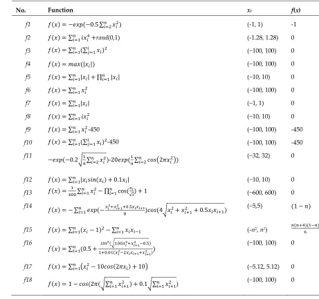
Table 1. The 18 standard benchmark functions (f1-f10 are the uni-modal, f11-f18 are the multi-modal functions).
306
No. Function xi f(x)
f1 ( ) = − (−0.5 ∑ ) (-1, 1) -1
f2 ( ) = ∑ +rand(0,1) (-1.28, 1.28) 0
f3 ( ) = ∑ (∑ ) (−100, 100) 0
f4 ( ) = (| |) (−100, 100) 0
f5 ( ) = ∑ | | + ∏ | | (−10, 10) 0
f6 ( ) = ∑ (−100, 100) 0
f7 ( ) = ∑ | | (−1, 1) 0
f8 ( ) = ∑ (−10, 10) 0
f9 ( ) = ∑ -450 (−100, 100) -450
f10 ( ) = ∑ (∑ )-450 (−100, 100) -450
f11
− (−0.2 ∑ )-20 ( ∑ 2 ) (−32, 32) 0
f12 ( ) = ∑ | ( ) + 0.1 | (−10, 10) 0
f13 ( ) = ∑ − ∏ cos (√) + 1 (−600, 600) 0
f14
( ) = − ∑ (− . ) (4 + + 0.5 ) (−5,5) (1 − )
f15 ( ) = ∑ ( − 1) − ∑ (-n2, n2) ( )( )
f16
( ) = ∑ (0.5 + ( . )
. ( ))
(−100, 100) 0
f17 ( ) = ∑ − 10 (2 ) + 10 (−5.12, 5.12) 0
f18
( ) = 1 − (2 ( ∑ ) + 0.1 ∑ ) (−100, 100) 0
307
308
309
310
311
312
313
314
Table 2. Summary of the CEC’17 benchmark test functions (search range = [-100, 100], dimension = 50 and 100).
316
Function Type Function Name Optimum
f1 Uni-modal Shifted and Rotated Bent Cigar Function 100
f2 Uni-modal Shifted and Rotated Sum of Different Power Function 200
f3 Uni-modal Shifted and Rotated Zakharov Function 300
f4 Simple multi-modal Shifted and Rotated Rosenbrock’s Function 400
f5 Simple multi-modal Shifted and Rotated Rastrigin’s Function 500
f6 Simple multi-modal Shifted and Rotated Expanded Scaffer’s F6 Function 600
f7 Simple multi-modal Shifted and Rotated Lunacek Bi_Rastrigin Function 700
f8 Simple multi-modal Shifted and Rotated Non-Continuous Rastrigin’s Function 800
f9 Simple multi-modal Shifted and Rotated Levy Function 900
f10 Simple multi-modal Shifted and Rotated Schwefel’s Function 1000
f11 Hybrid Functions Hybrid Function 1 (N=3) 1100
f12 Hybrid Functions Hybrid Function 2 (N=3) 1200
f13 Hybrid Functions Hybrid Function 3 (N=3) 1300
f14 Hybrid Functions Hybrid Function 4 (N=4) 1400
f15 Hybrid Functions Hybrid Function 5 (N=4) 1500
f16 Hybrid Functions Hybrid Function 6 (N=4) 1600
f17 Hybrid Functions Hybrid Function 6 (N=5) 1700
f18 Hybrid Functions Hybrid Function 6 (N=5) 1800
f19 Hybrid Functions Hybrid Function 6 (N=5) 1900
f20 Hybrid Functions Hybrid Function 6 (N=6) 2000
f21 Composition Functions Composition Function 1 (N=3) 2100
f22 Composition Functions Composition Function 2 (N=3) 2200
f23 Composition Functions Composition Function 3 (N=4) 2300
f24 Composition Functions Composition Function 4 (N=4) 2400
f25 Composition Functions Composition Function 5 (N=5) 2500
f26 Composition Functions Composition Function 6 (N=5) 2600
f27 Composition Functions Composition Function 7 (N=6) 2700
f28 Composition Functions Composition Function 8 (N=6) 2800
f29 Composition Functions Composition Function 9 (N=3) 2900
f30 Composition Functions Composition Function 10 (N=3) 3000
317
318
Table 3. The initial parameters of the FOA variants.
320
Algorithm Strategy Reference
FOA A new Fruit Fly Optimization Algorithm: Taking the financial distress model as an example
Pan [40]
LGMS LGMS-FOA: An Improved Fruit Fly Optimization Algorithm for Solving Optimization Problems
Shan [11]
IFFO An improved fruit fly optimization algorithm for continuous function optimization problems
Pan [12]
MFOA On a novel multi-swarm fruit fly optimization algorithm and its application
Yuan [14]
MSFOA A novel multi-scale cooperative mutation fruit fly optimization algorithm Zhang [26] CEFOA Novel fruit fly optimization algorithm with trend search and co-evolution Han [27]
Table 4. The initial parameters of the six meta-heuristic algorithms.
321
Algorithm Strategy Reference
PSO Particle swarm optimization Kennedy [1]
DE Differential Evolution – A Simple and Efficient Heuristic for global Optimization over Continuous Spaces
Storn [9]
GSA GSA: A Gravitational Search Algorithm Rashedi [41]
HS A new meta-heuristic algorithm for continuous engineering optimization: harmony search theory and practice
Lee [42]
BA A New Metaheuristic Bat-Inspired Algorithm Yang [5]
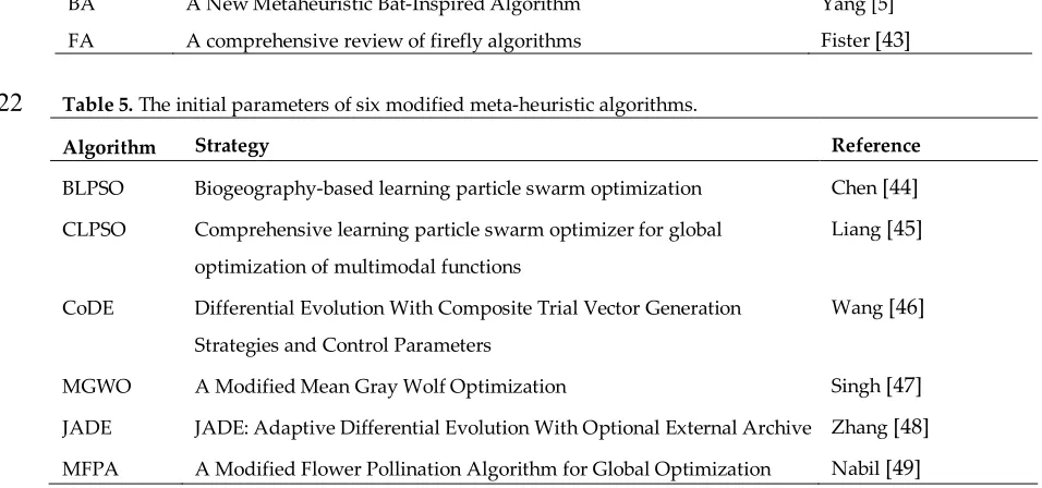
FA A comprehensive review of firefly algorithms Fister [43]
Table 5. The initial parameters of six modified meta-heuristic algorithms.
322
Algorithm Strategy Reference
BLPSO Biogeography-based learning particle swarm optimization Chen [44]
CLPSO Comprehensive learning particle swarm optimizer for global optimization of multimodal functions
Liang [45]
CoDE Differential Evolution With Composite Trial Vector Generation Strategies and Control Parameters
Wang [46]
MGWO A Modified Mean Gray Wolf Optimization Singh [47]
JADE JADE: Adaptive Differential Evolution With Optional External Archive Zhang [48]
MFPA A Modified Flower Pollination Algorithm for Global Optimization Nabil [49]
323
324
325
4. The Experiments and Evaluations
327
There are three groups of competitive algorithms. The first group, shown in Table 3, is the FOA
328
variants including FOA, LGMS, IFFO, MFOA, MSFOA, and CEFOA. The second group, shown in
329
Table 4, comprise of CEFOA and six meta-heuristic algorithms; PSO, DE, GSA, HS, BA, and FA. The
330
third group, shown in Table 5, comprise of CEFOA and six other meta-heuristic algorithms; BLPSO,
331
CLPSO, CoDE, JADE, MGWO, and MFPA.
332
The performances of the proposed algorithm and that of the competitive algorithms are
333
evaluated through two groups of benchmark functions; 18 scalable functions taken from [27] and 30
334
complex functions taken from CEC’2017 [50]. The definition of the functions in the first group and
335
their global optima are listed in Table 1; f1 - f10 are the uni-modal functions, and f11 - f18 are the
336
multi-modal functions. Table 2 showed the details of CEC’2017 functions; f1 - f3 are the uni-modal
337
functions, f4 - f10 are the simple multi-modal functions, f11 - f20 are the hybrid functions and f21 - f30
338
are the composite functions, respectively. The CEC’ 2017 benchmark functions are very challenging
339
as they are harder than that from the first problems set.
340
The experimental environment is MATLAB 9.2.0 (R2017a) that ran on a personal computer with
341
a 3.2 GHz CPU, 8 GB RAM. The operating system is Microsoft Windows 7 operating system (64-bit).
342
4.1 Parameters and Settings
343
There are three experiments, each of which is as follows.
344
1. The first experiment, the proposed CPFOA is compared with the competitive algorithms from
345
the first group, i.e., CPFOA and the FOA variants are competing. The comparison is conducted on
346
the 18 scalable functions taken from [27]. The dimension of each problem is set to three values; 30, 50,
347
and 1000.
348
2. The second experiment, the proposed CPFOA is compared with the competitive algorithms
349
from the second group, i.e., CPFOA and the original version of some state-of-the-art algorithms are
350
competing. The comparison is based on the 18 scalable functions taken from [27]. The dimension of
351
each problem is set as of the first experiment.
352
3. The third experiment, the proposed CPFOA is compared with the competitive algorithms from
353
the third group, i.e., CPFOA and more recent challenging algorithms are competing. The
354
comparison is conducted on 30 scalable functions taken from CEC’2017 [50]. The dimension of each
355
problem is set to two values; 50 and 100.
356
The following settings are set to comply with that of the existing CEFOA; the maximum
357
iteration ( _ ) of each algorithm is fixed to 500, the population sizes (popsize) is 30, and the
358
average (ave) and the standard deviations (std) of the final objective values are computed from 50
359
replications. The other parameters of each competitive algorithm are set in accordance with their
360
original literature, which are listed in Table 3, Table 4 and Table 5.
361
366
4.2 Performance Criteria
367
The criteria for performance evaluation of the competing algorithms are the quality, the
368
robustness, the success rate, and the statistical test, where each of which is as follow.
369
1. The quality of algorithms is determined by the average value (ave) and standard deviation (std)
370
of the final objective values. A lower value is better. Moreover, the decision can be supported by the
371
convergence graph.
372
2. The robustness of algorithm is presented by the boxplot diagram. The narrow box plot
373
represents a better distribution of final solution produced from algorithm.
374
3. The success rate (SR) determines by the number of successful runs over the total number of
375
runs. A run is a successful run if the algorithm finds a feasible solution x, represented by ( ) −
376
( ∗) ≤ 1 − 10, within the maximum number of function calls (the terminated condition of each
377
run( )), where x is a feasible optimal solution of the function, and ∗ is thebest known
378
solution of a specific problem f. A higher average indicates a better performance. The average
379
success rate ( ) is written as:
380
=number of successful runs total number of runs
(19)
4. Statistical test, to investigate the significant of difference between CPFOA’s outcome and the
381
competitive algorithm’s outcome, the Wilcoxon signed rank test with the significance level of 0.05
382
is conducted to judge whether the 50 runs of CPFOA are statistically better than that of another
383
competitor. The h values signifying the results of the Rank-sum test are indicated in Table 6 – 13 by
384
one of three symbols; “+”, “-” or “=”. Where the “+” symbol means that the solutions produced by
385
the competitive algorithm are better than, the “=” symbol means the outcomes of the competitive
386
algorithm are comparable to or similar to, and the “-” symbol means that the outcomes of the
387
competitive algorithm are worse than those of CPFOA. To conclude the statistical test, the total h is
388
represented as #1/#2/#3, where #1, #2, and #3 represents the number of wins, ties, and loss for the
389
algorithm, respectively.
390
5. Results and Discussion
391
5.1 Convergence Behavior of CPFOA
392
This section will provide consistent information about the convergence behavior of CPFOA
393
when the problem has an unknown number of local optima. The contours of the Egg holder function
394
[51] and Schaffer function [52] are plotted in Figure 4 and Figure 5, respectively. In addition, the
395
artificial fruit flies, appeared at several iterations, are also scattered in the different plots of the two
396
functions. The optimal points of the two functions are located at near the top right corner, and at the
397
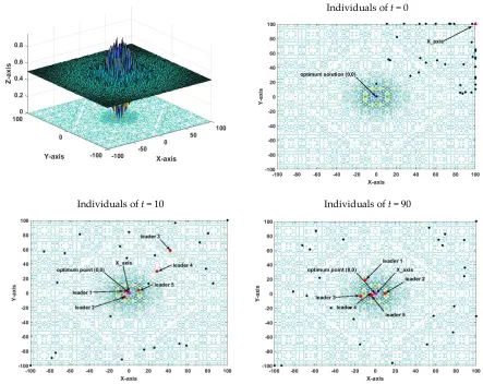
origin, respectively. The starting points are far from the optimal points. We have observed from
398
Figure 4 and Figure 5 that CPFOA has the capability of successfully optimizing the multimodal
399
functions without trapping in local optima. The experiment has been repeated for 50 runs and every
400
run reaches the optimal point. Now we can conclude that CPFOA has a balance between
401
diversification (diversification) and intensification (exploitation), since it has not trapped in local
402
Individuals of initial t = 0
Individuals of t = 10 Individuals of t = 125
Figure 4. Convergence behavior of CPFOA on Egg holder function.
404
405
406
407
408
409
Individuals of t = 0
Individuals of t = 10 Individuals of t = 90
Figure 5. Convergence behavior of CPFOA on Schaffer function.
411
412
413
414
415
416
417
418
419
420
421
422
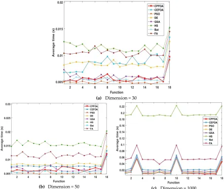
5.2 Computational Time of CPFOA
424
Optimization problem should be solved in short time. Therefore, a good meta-heuristic
425
optimization should have a short computational time. Figure 6 shows the average computational
426
time consumed by eights algorithms when they optimized 18 of the scalable functions taken from
427
[27]. From the figure, we found that CPFOA consumes quite short computational time compared to
428
the other algorithms, especially when the dimension of problem is 1000. Therefore, CPFOA can be
429
used effectively in optimizing a large scale problem.
430
(a) Dimension = 30
(b) Dimension = 50 (c) Dimension = 1000
Figure 6. Comparison of the average computational time from 50 runs based on 18 benchmark functions (500 iterations).
5.3 The First Experiment: Compare CPFOA to Six FOA Variants
431
The average (ave) and standard deviation (std) of the final objective values as well as h and SR
432
values produced by seven algorithms performing 18 benchmark functions with the dimension of
433
30, 50 and 1000 are shown in Table 6, 7, and 8, respectively. The algorithms having the lowest ave or
434
the lowest std in any case are highlighted in boldface. To conclude the table, the totals of h and
435
average of SR values are shown in the last rows.
436
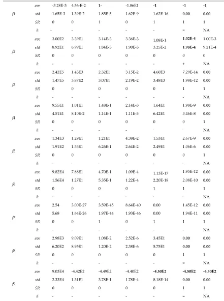
As can be seen from Table 6 and Table 7, CPFOA shows excellent performance with the total of
437
h is of 11/6/1; for the uni-modal functions f1- f10, it has 5 wins, 4 ties, and 1 loss, for the multi-modal
438
functions f11-f18, it has 6 wins, 2 ties, and 0 loss. Moreover, from the last row of Table 6 and 7,
439
For the large scale problem, the results are shown in Table 8. CPFOA still shows a very good
441
performance with the total of h is of 9/8/1; for the uni-modal functions f1- f10, it has 3 wins, 5 ties, and
442
1 loss, for the multi-modal functions f11-f18, it has 6 wins, 3 ties, and 0 loss. In addition, from the last
443
row of Table 8, CPFOA has the highest the average SR value (0.83).
444
To confirm the efficiency of the CPFOA, the convergence graphs of all seven algorithms when
445
they are optimizing 18 benchmark test functions with dimension = 1000 are shown in Figure 7,
446
where the red lines are the convergence graph of CPFOA. The graph is plotted in the log-log scale,
447
where the x-axis is the number of iterations, and the y-axis is the average fitness values obtained at
448
the corresponding iterations from the algorithms. From the graphs, CPFOA can reach the best
449
solution faster than the other six FOA variants.
450
The box plots can reveal the distribution of final objective values produced by the algorithms.
451
Figure 8 (a) is generated from f4, f5 (dimension = 30) and Figure 8 (b) is generated from f4, f5
452
(dimension = 50), Figure 8 (c) is generated from f4, f5 (dimension = 1000). These box plots reveal that
453
CPFOA is very robust to the increment of problem dimension as its final objective values
454
distribution is very narrow when the problem dimension increases.
455
Table 6. Solution quality comparisons of the CPFOA and variant FOAs performing 18 benchmark functions
483
(Dimension = 30). The h values signify the results of the Rank-sum test. The total h is represented as #1/#2/#3,
484
where #1, #2, and #3 represents the number of wins, ties, and loss for the algorithm, respectively. The SR is the
485
success rate. For each function, the lowest of ave and std values, and the highest of SR value are highlighted with
486
the boldfaces.
487
Function Criteria FOA LGMS IFFO MFOA MSFOA CEFOA CPFOA
f1
ave -3.28E-3 4.56 E-2 - 1 - -1.86E1 -1 -1 -1
std 1.65E-3 1.39E-2 1.85E-5 1.62E-9 1.62E-16 0.00 0.00
SR 0 0 1 0 1 1 1
h - - - = NA
f2
ave 3.00E2 3.39E1 3.14E-3 3.36E-3 1.08E-1 1.02E-4 1.00E-3
std 8.92E1 6.99E1 1.84E-3 1.90E-3 3.25E-2 1.98E-4 9.21E-4
SR 0 0 0 0 0 0 0
h - - - + NA
f3
ave 2.42E5 1.43E3 2.32E1 3.15E-2 4.60E3 7.29E-14 0.00
std 1.47E5 3.87E2 3.07E1 2.19E-2 3.48E3 1.98E-12 0.00
SR 0 0 0 0 0 1 1
h - - - NA
f4
ave 9.55E1 1.01E1 1.48E-1 2.14E-3 1.64E1 1.98E-9 0.00
std 4.51E1 8.10E-2 1.14E-1 1.11E-3 6.42E1 3.46E-8 0.00
SR 0 0 0 0 0 0 1
h - - - - - - NA
f5
ave 1.34E3 1.29E1 1.21E1 4.38E-2 1.53E1 2.67E-9 0.00
std 1.91E2 1.53E1 6.26E-1 2.64E-2 2.49E1 1.06E-6 0.00
SR 0 0 0 0 0 0 1
h - - - NA
f6
ave 9.82E4 7.88E1 4.70E-1 1.09E-4 1.13E-17 1.95E-12 0.00
std 1.56E4 1.27E1 5.35E-1 1.22E-4 2.20E-18 2.08E-10 0.00
SR 0 0 0 0 1 1 1
h - - - NA
f7
ave 2.54 3.00E-27 3.59E-45 8.64E-40 0.00 1.45E-12 0.00
std 5.68 1.64E-26 1.97E-44 1.93E-46 0.00 1.94E-11 0.00
SR 0 0 1 0 1 1 1
h - - - NA
f8
ave 2.98E3 9.09E1 1.08E-2 2.52E-6 3.45E1 0.00 0.00
std 6.20E2 8.95E1 1.20E-2 2.38E-6 5.75E1 0.00 0.00
SR 0 0 0 0 0 1 1
h - - - = NA
f9
ave 9.03E4 -4.42E2 -4.49E2 -4.40E2 -4.50E2 -4.50E2 -4.50E2
std 2.33E4 1.31E1 3.78E-1 1.78E-4 8.18E-14 0.00 0.00
SR 0 0 0 0 0 1 1
f10 ave 4.56E5 8.79E2 -4.48E2 -4.45E2 4.93E3 -4.50E2 -4.50E2
std 3.96E5 4.90E2 4.37E1 2.89E-2 3.44E3 0.00 0.00
SR 0 0 0 0 0 1 1
h - - - = NA
f11
ave 2.05E1 3.46E1 1.80E-1 1.43 2.76E1 1.60E-10 8.88E-16
std 1.84E-1 1.33E-1 1.34E-1 1.96 4.60E1 4.01E-10 0
SR 0 0 0 0 0 1 1
h - - - NA
f12
ave 6.96E1 6.78E1 1.56E-2 1.21 7.64E1 9.15E-14 0.00
std 1.20E1 6.26E-1 1.15E-2 2.70 2.92E1 1.55E-12 0.00
SR 0 0 0 0 0 1 1
h - - - NA
f13
ave 8.51E2 1.01E1 2.27E-1 1.52E-4 1.09E-02 8.89E-16 0.00
std 2.76E2 1.98E-2 2.57E-1 7.46E-5 1.29E-02 4.70E-15 0.00
SR 0 0 0 0 0 1 1
h - - - NA
f14
ave -3.17 1.80 E1 - 2.13 E1 - -2.14E1 -8.54E1 -2.73E1 -2.70E1
std 1.08 1.30E1 8.91E-1 2.82E-4 1.77E1 1.05 2.80E-2
SR 0 0 0 0 0 1 1
h - - - NA
f15
ave 6.04E6 -5.18E2 5.30E1 3.06E1 3.19E4 -1.89E4 -3.12E3
std 7.89E5 8.13E1 2.67E1 3.67E-1 2.82E4 3.60E3 5.79E1
SR 0 0 0 0 0 0 1
h - - - NA
f16
ave 1.33E1 8.40E1 9.12E-1 9.51E-7 1.23E1 0.00 0.00
std 4.26E-1 7.17E-1 2.71E-1 1.89E-6 3.84E-1 0.00 0.00
SR 0 0 0 0 0 1 1
h - - - = NA
f17
ave 4.19E2 4.19E2 1.17E-1 1.05E2 1.33E2 1.46E-8 0.00
std 5.27E1 2.06E1 1.58E-1 1.31E2 3.90E1 4.42E-8 0.00
SR 0 0 0 0 0 0 1
h - - - NA
f18
ave 3.72 6.60E-2 1.81E-4 9.99E-2 6.48E-14 0.00 0.00
std 3.90 4.97E-2 2.55E-4 3.45E-7 7.76E-14 0.00 0.00
SR 0 0 0 0 1 1 1
h - - - = NA
total
h
+ 0 0 0 0 0 1 11
- 18 18 18 18 18 11 1
= 0 0 0 0 0 6 6
Average SR 0.00 0.00 0.11 0.00 0.22 0.72 0.94
Table 7. Solution quality comparisons of the CPFOA and variant FOAs performing 18 benchmark functions
490
(Dimension = 50). The h values signify the results of the Rank-sum test. The total h is represented as #1/#2/#3,
491
where #1, #2, and #3 represents the number of wins, ties, and loss for the algorithm, respectively. The SR is the
492
success rate. For each function, the lowest of ave and std values, and the highest of SR value are highlighted with
493
the boldfaces.
494
Function Criteria FOA LGMS IFFO MFOA MSFOA CEFOA CPFOA
f1
ave -5.05E-4 4.17E-3 -1 -9.92E-1 -1 -1 -1
std 1.21E-4 2.44E-3 3.03E-5 3.18E-9 2.96E-8 0.00 0.00
SR 0 0 1 0 1 1 1
h - - - - - = NA
f2
ave 7.69E2 1.29E2 4.99E-03 3.80E-3 5.38E-1 9.52E-5 1.03E-3
std 1.09E2 1.76E1 3.39E-03 1.56E-3 1.88E-1 2.08E-4 8.76E-4
SR 0 0 0 0 0 0 0
h - - - - - + NA
f3
ave 1.22E6 6.49E3 4.12E1 7.52E-2 5.06E4 1.02E-13 0.00
std 1.03E6 1.68E3 4.45E1 3.17E-2 1.89E4 2.10E-12 0.00
SR 0 0 0 0 0 1 1
h - - - - - - NA
f4
ave 9.69E1 1.07E1 1.95E-1 1.26E-3 4.70E1 1.99E-9 0.00
std 2.37 7.91E-2 1.49E-1 2.08E-4 7.62E1 3.50E-8 0.00
SR 0 0 0 0 0 0 1
h - - - - - - NA
f5
ave 2.42E3 2.23E1 1.71E1 8.01E-2 1.64E2 1.97E-29 0.00
std 1.80E2 1.63E1 1.01E1 5.92E-2 6.57E1 1.01E-6 0.00
SR 0 0 0 0 0 1 1
h - - - - - - NA
f6
ave 1.59E5 1.53E1 2.08E-1 1.32E-4 8.76E-5 1.02E-12 0.00
std 1.73E4 1.90E 2.58E-1 1.14E-4 4.37E-4 1.88E-10 0.00
SR 0 0 0 0 1 1 1
h - - - - - - NA
f7
ave 2.57E-1 5.19E-53 2.91E-22 4.98E-44 0.00 1.95E-12 0.00
std 4.33E-1 2.84E-52 2.00E21 - 3.50E-43 0.00 1.48E-11 0.00
SR 0 1 1 0 1 1 1
h - - - - - - NA
f8
ave 9.81E3 2.82E2 2.57E-2 1.38E-5 6.24E1 0.00 0.00
std 3.15E3 2.27E1 4.39E-2 1.09E-5 4.80E1 0.00 0.00
SR 0 0 0 0 0 1 1
h - - - - - = NA
f9
ave 1.65E5 -4.46E2 -4.48E2 -4.45E2 -4.50E2 -4.50E2 -4.50E2
std 1.90E4 5.82E-1 2.23E 9.61E-5 1.88E-4 0.00 0.00
SR 0 0 0 0 1 1 1
f10 ave 3.51E6 -2.53E2 -2.60E1 -4.35E2 4.80E4 -4.50E2 -4.50E2
std 2.99E6 3.50E2 4.23E2 1.45E-1 1.64E4 0.00 0.00
SR 0 0 0 0 0 1 1
h - - - - - = NA
f11
ave 2.06E1 3.53E1 1.19E-1 2.50E-3 1.15E1 1.69E-10 8.88E-16
std 1.68E-1 1.12E-1 1.17E-1 6.19E-4 7.12E1 2.13E-10 0.00
SR 0 0 0 0 0 1 1
h - - - - - - NA
f12
ave 1.29E2 1.21E1 1.93E-2 1.57E-3 2.03E1 1.05E-15 0.00
std 1.71E1 9.39E-1 1.83E-2 7.03E-4 5.40E1 1.95E-13 0.00
SR 0 0 0 0 0 1 1
h - - - - - - NA
f13
ave 1.37E3 1.04E1 2.01E-1 2.47E-4 3.23E-2 1.09E-17 0.00
std 2.77E2 8.73E-3 2.05E-1 1.17E-4 1.55E-2 8.70E-14 0.00
SR 0 0 0 0 0 1 1
h - - - - - - NA
f14
ave -6.00 2.83 E1 - 3.38E1 -3.62E1 -1.27E1 -2.58E1 -4.45E1
std 1.80 1.41E1 1.15E1 3.77E-4 2.04E1 1.52 1.56
SR 0 0 0 0 0 0 1
h - - - - - - NA
f15
ave 8.73E7 1.03E3 3.90E8 5.47E1 9.22E5 -1.69E4 -8.60E3
std 2.00E7 5.99E2 5.16E8 2.60 4.47E5 2.64E3 2.02E2
SR 0 0 0 0 0 0 1
h - - - - - - NA
f16
ave 2.30E1 1.65E1 9.40E-1 1.12E-6 2.18E1 0.00 0.00
std 4.12E-1 9.15E-1 3.19E-1 1.38E-6 5.77E-1 0.00 0.00
SR 0 0 0 0 0 1 1
h - - - - - = NA
f17
ave 7.63E2 9.15E2 1.92E-1 4.01E-5 1.47E4 1.06E-8 0.00
std 6.98E1 3.24E1 1.95E-1 3.32E-5 2.21E2 2.27E-8 0.00
SR 0 0 0 0 0 0 1
h - - - - - - NA
f18
ave 2.14 3.53E-2 1.60E-4 9.99E-2 6.47E-14 0.00 0.00
std 3.72 4.68E-2 2.51E-4 2.09E-6 6.24E-14 0.00 0.00
SR 0 0 0 0 1 1 1
h - - - - - = NA
total
h
+ 0 0 0 0 0 1 11
- 18 18 18 18 18 11 1
= 0 0 0 0 0 6 6
Average SR 0.00 0.05 0.11 0.00 0.27 0.72 0.94
Table 8. Solution quality comparisons of the CPFOA and variant FOAs performing 18 benchmark functions
497
(Dimension = 1000). The h values signify the results of the Rank-sum test. The total h is represented as #1/#2/#3,
498
where #1, #2, and #3 represents the number of wins, ties, and loss for the algorithm, respectively. The SR is the
499
success rate. For each function, the lowest of ave and std values, and the highest of SR value are highlighted with
500
the boldfaces.
501
Function Criteria FOA LGMS IFFO MFOA MSFOA CEFOA CPFOA
f1
ave -1.87E-35 7.20E-62 -1.00 -9.98E-6 -3.14E-54 -1 -1
std 4.74E-35 8.73E-62 1.62E-4 2.07E-06 8.37E-54 0.00 0.00
SR 0 0 0 0 0 1 1
h - - - - - = NA
f2
ave 4.01E5 7.36E4 2.21E-2 1.24E-2 1.60E5 0.00 2.53E-4
std 1.85E4 2.29E3 1.28E-2 4.92E-3 5.16E3 0.00 2.55E-4
SR 0 0 0 0 0 1 0
h - - - - - + NA
f3
ave 1.24E9 7.01E7 4.96E2 5.33E3 3.26E7 0.00 0.00
std 1.16E9 3.02E6 7.53E2 4.70E3 9.74E6 0.00 0.00
SR 0 0 0 0 0 1 1
h - - - - - = NA
f4
ave 9.99E1 1.36E1 1.49E-1 4.71E-3 9.71E1 1.80E-9 0.00
std 1.90E-1 1.47E-2 1.10E-1 1.91E-3 5.75E-1 1.06E-8 0.00
SR 0 0 0 0 0 0 1
h - - - - - - NA
f5
ave 4.98E4 5.02E2 1.12E1 4.45 4.13E3 0.00 0.00
std 8.52E2 1.01E1 8.06E1 3.26 6.01E1 0.00 0.00
SR 0 0 0 0 0 1 1
h - - - - - = NA
f6
ave 3.35E6 3.67E2 2.34E1 1.98E-2 2.53E6 1.74E-12 0.00
std 7.07E4 8.96E1 3.61E1 2.50E-2 4.64E4 3.28E-10 0.00
SR 0 0 0 0 0 1 1
h - - - - - - NA
f7
ave 1.92 0.00 0.00 7.57E-1 0.00 1.15E-13 0.00
std 1.11 0.00 0.00 1.88E-5 0.00 1.72E-11 0.00
SR 0 1 1 0 1 1 1
h - = = - = - NA
f8
ave 4.46E6 1.41E5 2.97E1 3.66E-2 3.06E6 0.00 0.00
std 8.13E4 2.37E3 3.97E1 3.60E-2 7.01E4 0.00 0.00
SR 0 0 0 0 0 1 1
h - - - - - = NA
f9
ave 3.35E6 -3.66E2 -4.48E2 -4.40E2 2.52E6 -4.50E2 -4.50E2
std 7.25E4 3.21E1 2.23E1 2.05E-2 5.85E4 0.00 0.00
SR 0 0 0 0 0 1 1
f10 ave 1.57E9 6.34E5 4.23E2 4.66E3 7.77E6 -4.50E2 -4.50E2
std 2.72E9 1.14E6 1.22E2 4.36E3 3.64E4 0.00 0.00
SR 0 0 0 0 0 1 1
h - - - - - = NA
f11
ave 2.11E1 3.81E1 5.96E-2 2.86 2.07E1 7.64E-11 8.88E-16
std 2.71E-2 1.60E-2 5.02E-2 1.59 2.66E-2 2.00E-10 0.00
SR 0 0 0 0 0 1 1
h - - - - - - NA
f12
ave 2.93E3 3.06E2 2.00E-1 3.01E-2 2.18E3 1.15E-14 0.00
std 4.12E1 3.75E1 1.58E-1 1.41E-2 5.35E1 1.51E-12 0.00
SR 0 0 0 0 0 1 1
h - - - - - - NA
f13
ave 2.96E4 1.81E1 1.76E-1 3.16E-3 2.26E4 2.09E-16 0.00
std 8.47E2 1.98E-2 2.08E-1 1.40E-3 4.17E2 3.79E-15 0.00
SR 0 0 0 0 0 1 1
h - - - - - - NA
f14
ave -2.31E1 4.52E2 -5.29E2 -7.37E2 -1.11E2 -2.32E1 -9.23E2
std 3.91E1 8.21E1 6.83E 8.41E-3 1.29E1 1.05 6.45
SR 0 0 0 0 0 0 0
h - - - - - - NA
f15
ave 3.37E14 8.36E9 3.90E8 1.00E5 2.23E14 -1.29E4 -1.02E6
std 1.29E13 3.83E8 5.16E8 3.39E4 6.18E12 2.54E3 1.64E3
SR 0 0 0 0 0 0 0
h - - - - - - NA
f16
ave 4.89E2 4.63E2 3.25E1 3.86E-4 4.78E2 0.00 0.00
std 1.14E1 3.87E1 4.74E1 7.92E-4 4.52E1 0.00 0.00
SR 0 0 0 0 0 1 1
h - - - - - = NA
f17
ave 1.79E4 1.02E4 1.39E1 7.96E2 1.47E4 1.14E-8 0.00
std 3.77E2 1.15E2 1.25E1 4.45E2 1.61E2 3.27E-8 0.00
SR 0 0 0 0 0 0 1
h - - - - - - NA
f18
ave 3.93E1 4.05E-2 1.02E-4 9.99E-2 9.33E-14 0.00 0.00
std 3.99E1 4.73E-2 9.30E-5 1.88E-5 9.48E-14 0.00 0.00
SR 0 0 0 0 0 1 1
h - - - - - = NA
total
h
+ 0 0 0 0 0 1 9
- 18 17 17 18 17 9 1
= 0 1 1 0 1 8 8
Average SR 0.00 0.05 0.05 0.00 0.05 0.77 0.83
Figure 7. Convergence curves of 18 benchmark functions that compare CPFOA, CEFOA, FOA, LGMS, IFFO, MFOA and MSFOA. The dimension of problem is 1000.
504
(a) Dimension = 30
(c) Dimension = 1000
Figure 8. Box plots of the optimal solutions which evaluated from standard benchmark function f4 and f5 (1=CPFOA, 2=CEFOA, 3=FOA, 4=LGMS, 5=IFFO, 6=MFOA, 7=MSFOA).
5.4 The Second Experiment: Comparison of the CPFOA and Meta-Heuristics Algorithms
505
This section presents a comparison of the CPFOA to the six meta-heuristics algorithms: PSO,
506
DE, GSA, HS, BA, FAand including CEFOA. The average (ave) and standard deviation (std) of the
507
final objective values as well as h and SR values produced by the competitive algorithms
508
performing 18 benchmark functions with the dimension of 30, 50 and 1000 are shown in Table 9, 10,
509
and 11, respectively. To conclude the table, the totals of h and average of SR values are shown in the
510
last rows.
511
Table 9 and Table 10, CPFOA shows the best performance with the total of h is of 11/6/1; for
512
the uni-modal functions f1- f10, it has 5 wins, 4 ties, and 1 loss, for the multi-modal functions f11-f18,
513
it has 6 wins, 2 ties, and 0 loss. Moreover, from the last row of Table 9 and 10 CPFOA has the highest
514
the average SR value (0.94).
515
For the large scale problem set, the results are shown in Table 11. CPFOA still shows a very
516
promising performance with the total of h is of 9/8/1; for the uni-modal functions f1- f10, it has 3
517
wins, 6 ties, and 1 loss, for the multi-modal functions f11-f18, it has 6 wins, 2 ties, and 0 loss. In
518
addition, from the last row of Table 11, CPFOA has the highest the average SR value (0.83).
519
Table 9. Solution quality comparisons of the CPFOA and the meta-heuristic algorithms performing 18
532
benchmark functions (Dimension = 30). The h values signify the results of the Rank-sum test. The total h is
533
represented as #1/#2/#3, where #1, #2, and #3 represents the number of wins, ties, and loss for the algorithm,
534
respectively. The SR is the success rate. For each function, the lowest of ave and std values, and the highest of SR
535
value are highlighted with the boldfaces.
536
Function Criteria PSO DE GSA HS BA FA CEFOA CPFOA
f1
ave -0.99 -1 -1 -9.83E-1 -1 -9.99E-1 -1 -1
std 3.75E-3 0.00 0.00 4.11E-3 1.51E-6 6.34E-4 0.00 0.00
SR 0.03 0.73 1 0 1 0 1 1
h - = = - = - = NA
f2
ave 7.94E-2 2.12E-1 8.34E-2 1.99E-1 9.95E1 3.59E-2 1.02E-4 1.00E-3
std 4.07E-2 8.95E-2 3.02E-2 5.29E-2 5.92E1 1.86E-2 1.98E-4 9.21E-4
SR 0 0 0 0 0 0 0 0
h - - - - - - + NA
f3
ave 8.28E2 6.89E2 9.49E2 2.11E4 5.29E4 1.16E3 7.29E-14 0.00
std 1.05E3 4.97E2 3.11E2 5.78E3 2.27E4 4.47E2 1.98E-12 0.00
SR 0 0 0 0 0 0 1 1
h - - - - - - - NA
f4
ave 1.59E1 2.65E1 7.15E1 2.25E1 5.18E1 8.37E-2 1.98E-9 0.00
std 7.79E1 6.47E1 2.41E1 2.34E 7.41E1 1.84E-2 3.46E-8 0.00
SR 0 0 0 0 0 0 0 1
h - - - - - - - NA
f5
ave 1.87E2 1.18E1 1.95E2 1.81E1 5.41E33 1.51E1 2.67E-9 0.00
std 1.26E2 3.90E1 4.77E1 4.22E 2.27E34 2.13E1 1.06E-6 0.00
SR 0 0 0 0 0 0 0 1
h - - - - - - - NA
f6
ave 1.65E2 7.90E1 7.94E-3 3.21E2 2.12E4 5.71E-3 1.95E-12 0.00
std 2.30E2 1.98E1 4.35E-2 8.92E1 5.47E3 2.43E-3 2.08E-10 0.00
SR 0 0 0 0 0 0 1 1
h - - - - - - - NA
f7
ave 0.00 0.00 0.00 0.00 0.00 0.00 1.45E-12 0.00
std 0.00 0.00 0.00 0.00 0.00 0.00 1.94E-11 0.00
SR 1 1 1 1 1 1 1 1
h = = = = = = - NA
f8
ave 3.20E1 5.23E-1 3.10E-15 8.23E1 2.51E2 3.89E-1 0.00 0.00
std 5.52E1 1.79E1 1.90E-15 1.97E1 1.38E2 4.01E-1 0.00 0.00
SR 0 0.03 1 0 0 0 1 1
h - - - - - - = NA
f9
ave -3.37E2 -4.37E2 -4.50E2 -1.40E2 1.93E4 -4.50E2 -4.50E2 -4.50E2
std 1.14E2 3.08E1 3.17E-14 5.78E1 7.05E3 2.30E-3 0.00 0.00
SR 0.3 0.96 0 0 0 0 1 1
![Table 2. Summary of the CEC’17 benchmark test functions (search range = [-100, 100], dimension = 50 and 100)](https://thumb-us.123doks.com/thumbv2/123dok_us/8019200.1333608/12.595.64.524.94.691/table-summary-cec-benchmark-functions-search-range-dimension.webp)