The
K
L-
K
SMass Difference
ZiyuanBai1,Norman H.Christ1, andChristopher T.Sachrajda2,
1Physics Department, Columbia University, New York, NY 10027, USA
2Department of Physics and Astronomy, University of Southampton, Southampton SO17 1BJ, UK
Abstract. We review the status of the RBC-UKQCD collaborations’ computations of theKL-KS mass difference. After a brief discussion of the theoretical framework which
had been developed previously by the collaboration, we describe our latest computation, performed at physical quark masses, and present our preliminary result mKL −mKS =
(5.5±1.70)×10−12MeV.
1 Introduction
The value of theKL-KS mass difference,∆mK≡mKL−mKS =3.483(6)×10−12MeV, is truly tiny on
the scale ofΛQCD. Thisflavour-changing neutral current(FCNC) process is therefore an excellent
one in which to search for the effects of new physics. For example if we imagine an effective
new-physics∆S = 2 contribution of the form Λ12( ¯s· · ·d)( ¯s· · ·d), where the ellipses represent possible
Dirac matrices, and if we could reproduce the experimental∆mKin the SM to 10% accuracy then we
would be sensitive to scalesΛ>∼(103−104) TeV. This illustrates the sensitivity of precision flavour
physics to scales which are unreachable directly at the Large Hadron Collider.
The mass difference∆mKis obtained from second order weak perturbation theory, specifically:
∆mK≡mKL−mKS =2P
α
K¯0|H
W|α α|HW|K0 mK−Eα
=3.483(6)×10−12MeV, (1)
where the sum over the intermediate states|αincludes an integration over the relevant phase-space andHWis the effective weak Hamiltonian density.
The calculation of∆mK is one component of the RBC-UKQCD collaborations’ programme of
computations of long-distance contributions in kaon physics, requiring the evaluation of matrix ele-ments of bilocal operators of the form
d4x f|TQ
1(x)Q2(0)|i. (2)
Other applications being studied include the rare-kaon decaysK→π+−[1,2] andK+→π+νν¯[3,4]
and the indirect CP-violation parameterK[5]. Progress on all these topics is summarised by X. Feng
at this conference [6]. As well as computing the non-perturbative long-distance contributions from scales ofO(ΛQCD), we aim to avoid the necessity of performing perturbation theory at the scale ofmc.
1.1 Status of earlier RBC-UKQCD calculations of∆mK
Before presenting our new results we briefly summarise our previous work. In [8] we developed the framework necessary for the calculation of∆mK as well as performing an exploratory calculation
on a 163 ×32 lattice with unphysical masses (m
π = 421 MeV) and including only the connected
diagrams. However, the results were encouragingly, and perhaps surprisingly, reasonably close to the experimental value. This was followed by a calculation of all the diagrams on a 243×64 lattice with
inverse lattice spacinga−1 =1.729(28) GeV and with the unphysical massesm
π =330 MeV,mK =
575 MeV,mMS
c (2 GeV)=949 MeV [9]. For these parameters we found∆mK=3.19(41)(96) MeV. In this talk we will present an update of the computations and preliminary results obtained at physical masses.
2 The theoretical framework
K0 K¯0
ti tf
n
HW HW
tA tB
t1 t2
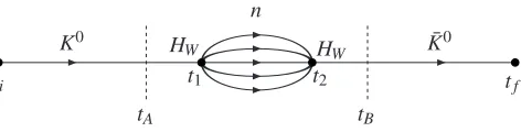
Figure 1.Representation of the four-point correlation functionC4from which∆mKis determined.
In this section we briefly review the theoretical framework used in the computation of∆mK[8,9].
In fig.1we sketch the four-point correlation function used to determine∆mK. TheK0( ¯K0) is created
(annihilated) atti (tf) and the two weak effective Hamiltonians are inserted at timest1,2 which are
integrated over the interval (tA,tB). With all the states at rest, the correlation function is given by
C4(tA,tB;ti,tf)=|ZK|2e−mK(tf−ti)
n
K¯0|H
W|n n|HW|K0
(mK−En)2
e(mK−En)T−(m
K−En)T −1
, (3)
whereT = tB−tA +1,ZK = K0|φ†K(0)|0andφ†K is the interpolating operator used to create the
kaon. From the coefficient ofT in eq.(3) we obtain
∆mFVK ≡2 n
K¯0|H
W|n n|HW|K0
(mK−En) , (4)
which should be compared to the infinite-volume expression in eq.(1). The superscriptFVin∆mFVK
stands for Finite Volume. The finite-volume corrections necessary to relate∆mFVK in (4) to∆mKin (1)
have been derived in [10].
The presence of terms in eq. (3) which grow exponentially withT when there are intermediate states|nwith energiesEnwhich are smaller thanmKis a generic feature of the calculation of matrix
elements of bilocal operators. The freedom to add terms of the formcSsd¯ andcPsγ¯ 5d, wherecS,P
are constants, toHW without changing∆mKallows us to remove two such contributions. We choose cP such that 0|HW +cPs¯γ5d|K0 = 0. A natural choice for cS would be such as to remove the
single-pion intermediate state. However, althoughmη >mK, the contribution from theηis noisy and
we find it numerically advantageous to eliminate this contribution. We therefore chosecS such that
η|HW+cSsd¯ |K0=0. This leaves us the single-pion and two-pion states to evaluate using three-point
1.1 Status of earlier RBC-UKQCD calculations of∆mK
Before presenting our new results we briefly summarise our previous work. In [8] we developed the framework necessary for the calculation of ∆mK as well as performing an exploratory calculation
on a 163 ×32 lattice with unphysical masses (m
π = 421 MeV) and including only the connected
diagrams. However, the results were encouragingly, and perhaps surprisingly, reasonably close to the experimental value. This was followed by a calculation of all the diagrams on a 243×64 lattice with
inverse lattice spacinga−1 =1.729(28) GeV and with the unphysical massesm
π =330 MeV,mK =
575 MeV,mMS
c (2 GeV)=949 MeV [9]. For these parameters we found∆mK=3.19(41)(96) MeV. In this talk we will present an update of the computations and preliminary results obtained at physical masses.
2 The theoretical framework
K0 K¯0
ti tf
n
HW HW
tA tB
t1 t2
Figure 1.Representation of the four-point correlation functionC4from which∆mKis determined.
In this section we briefly review the theoretical framework used in the computation of∆mK[8,9].
In fig.1we sketch the four-point correlation function used to determine∆mK. TheK0( ¯K0) is created
(annihilated) atti (tf) and the two weak effective Hamiltonians are inserted at timest1,2 which are
integrated over the interval (tA,tB). With all the states at rest, the correlation function is given by
C4(tA,tB;ti,tf)=|ZK|2e−mK(tf−ti)
n
K¯0|H
W|n n|HW|K0
(mK−En)2
e(mK−En)T−(m
K−En)T −1
, (3)
whereT = tB−tA +1, ZK =K0|φ†K(0)|0 andφ†K is the interpolating operator used to create the
kaon. From the coefficient ofT in eq.(3) we obtain
∆mFVK ≡2 n
K¯0|H
W|n n|HW|K0
(mK−En) , (4)
which should be compared to the infinite-volume expression in eq.(1). The superscriptFVin∆mFVK
stands for Finite Volume. The finite-volume corrections necessary to relate∆mFVK in (4) to∆mKin (1)
have been derived in [10].
The presence of terms in eq. (3) which grow exponentially withT when there are intermediate states|nwith energiesEnwhich are smaller thanmKis a generic feature of the calculation of matrix
elements of bilocal operators. The freedom to add terms of the formcSsd¯ andcPsγ¯ 5d, where cS,P
are constants, toHW without changing∆mKallows us to remove two such contributions. We choose cP such that 0|HW+cPs¯γ5d|K0 = 0. A natural choice for cS would be such as to remove the
single-pion intermediate state. However, althoughmη >mK, the contribution from theηis noisy and
we find it numerically advantageous to eliminate this contribution. We therefore chosecS such that
η|HW+cSsd¯ |K0=0. This leaves us the single-pion and two-pion states to evaluate using three-point
functions and to remove the corresponding growing exponentials.
d u,c s
s u,c d
K0 K¯0
Type 1
d
u,c s
s
u,c
d
K0 K¯0
Type 4
K0 K¯0
Type 2
s
s d
d u,c
u,c K
0 K¯0
Type 3
s
s d
d u,c
u,c
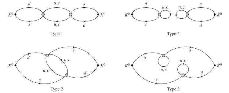
Figure 2. The four types of diagram contributing to theK0 →K¯0transition. The shaded circles represent the
insertion of the effective weak Hamiltonian.
2.1 Ultraviolet divergences in the calculation of∆mK
The∆S =1 effective Weak Hamiltonian takes the form:
HW =G√F
2
q,q=u,c
VqdVq∗s(C1Qqq
1 +C2Qqq
2 ) (5)
where the{Qqqi }i=1,2are current-current operators, defined as:
Q1qq=( ¯siγµ(1−γ5)di) (¯qjγµ(1−γ5)qj) and Q2qq=( ¯siγµ(1−γ5)dj) (¯qjγµ(1−γ5)qi). (6)
As the separation between the twoHWoperators decreases, we have the potential of new ultraviolet
divergences. The diagrams contributing to theK0- ¯K0transition correlation function are presented in
fig.2. Consider for example the Type1 diagram. Power counting suggests that the contribution from theu-quark in the central loop would lead to a quadratic divergence. However, theV −A nature of the currents together with the GIM mechanism leads to the elimination of both the quadratic and logarithmic divergences. Thus once the local operators Q1,2 are renormalised, no new ultraviolet
divergences arise. This is not the case forK or forK → πνν¯ rare kaons decays, where additional
divergences are present and need to be renormalised [3].
3 Details of the simulation
The calculation is being performed on aL3×T×L
s=643×128×12 lattice, using Möbius Domain
Wall Fermions and the Iwasaki gauge action; more details about the ensemble can be found in [11]. The inverse lattice spacinga−1=2.359(7) GeV and the light and strange quark masses correspond to
mπ =135.9(3) MeV andmK =496.9(7) MeV (very close to the physical masses of the neutral pion mπ0=134.98 MeV and kaonmK0=497.6 MeV). In studies of charm physics on these configurations,
the bare mass of the charm quark was determined to lie in the rangeamc 0.32 - 0.33. Our results
presented below were obtained usingamc = 0.31, but we have also studied the dependence onmc
finding it to be mild when compared to the overall uncertainties (see tables1and2below).
for each such diagram there are 4 contractions which need to evaluated, and we distinguish three types of quark propagators used in their evaluation.
1. We use Coulomb-gauge wall-source propagators for thedandsquarks at theK0source and ¯K0
sink on each time slice. Thed-quark propagators are obtained using standard low-mode deflation techniques. The lowest 2000 eigenvalues and the corresponding eigenvectors are obtained using the Lanczos algorithm. The full propagators are then obtained using the conjugate gradient algorithm, with asloppy stopping residual of 10−4 on all configurations and an exactone of 10−8 on a small
subset of configurations. These sloppy and exact propagators are used in theall mode averaging
(AMA) [12] procedure, as described below. For thes-quark propagator we simply use the conjugate gradient algorithm.
2. For the connected diagrams, i.e.those of type 1 and 2, on each time slice we generate point-source propagators at a single spacial point which corresponds to the position of one of the weak operators in fig.2. The spacial position of the source is varied from time-slice to time-slice; specifically for time slice 0<t <127, the source is placed at the point (4t(moduloL),4t(moduloL),4t(moduloL)).
These propagators connect to the position of the second insertion of the weak Hamiltonian, which is summed over all space so that momentum is conserved.
The point-source propagators for the uquark are also determined using low-mode deflation as described above. However, as explained below, they are only used in measurements of type 1 and 2 diagrams with exact propagators and so are only computed for a small subset of configurations. The point-sourcec-quark propagators are determined using the conjugate-gradient algorithm.
3. For theu-quark self-loops in the diagrams of type 3 and 4 we use the 2000 low-mode eigenvectors and eigenvalues mentioned above and complete the construction of the all-to-all propagators stochas-tically using 60 random space-time volume sources for each configuration. For thec-quark in these loops, the propagators are obtained stochastically with the same random sources as for theuquarks.
The preliminary results presented below were obtained on a subset of 59 configurations for the noisier type-3 and type-4 diagrams, using AMA withsloppypropagators corrected by including mea-surements with exact propagators on a subset of 7 configurations. The less noisy type-1 and type-2 diagrams were calculated on 11 configurations with exact stopping conditions for the propagators. An indication of the computational cost is about 5 hours on a 8K BG/Q machine for each sloppy
measure-ment and 15 hours for an exact one. The contributions from the different diagrams are combined and
the uncertainties are determined using the superjacknife procedure [13]. In addition, for the discon-nected type 4 diagrams, which are the most noisy, the left and right-hand sides, see Fig.2, are stored separately for theK0source and ¯K0sink in order to enable us to vary the source-sink separation. For
the diagrams of type 1, 2 and 3 the positions of theK0source and ¯K0sink are varied over all values
oftiandtf but their separationtf−tiis fixed to be 48.
4 Preliminary Results
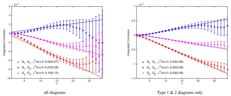
In the left-hand plot of fig.3we show the integrated correlation functions as a function ofT for each pair of operators (Qi,Qj) (i,j = 1,2). The mass difference∆mK is obtained from the slope of the
correlation function withT and in the figure we obtain the slopes by fitting the correlation function in the range 10≤T ≤20. From the slopes we obtain∆mFVK =(5.8±1.7) 10−12MeV. We now make a
for each such diagram there are 4 contractions which need to evaluated, and we distinguish three types of quark propagators used in their evaluation.
1. We use Coulomb-gauge wall-source propagators for thed andsquarks at theK0source and ¯K0
sink on each time slice. Thed-quark propagators are obtained using standard low-mode deflation techniques. The lowest 2000 eigenvalues and the corresponding eigenvectors are obtained using the Lanczos algorithm. The full propagators are then obtained using the conjugate gradient algorithm, with asloppy stopping residual of 10−4 on all configurations and anexact one of 10−8 on a small
subset of configurations. These sloppy and exact propagators are used in theall mode averaging
(AMA) [12] procedure, as described below. For thes-quark propagator we simply use the conjugate gradient algorithm.
2. For the connected diagrams, i.e.those of type 1 and 2, on each time slice we generate point-source propagators at a single spacial point which corresponds to the position of one of the weak operators in fig.2. The spacial position of the source is varied from time-slice to time-slice; specifically for time slice 0<t<127, the source is placed at the point (4t(moduloL),4t(moduloL),4t(moduloL)).
These propagators connect to the position of the second insertion of the weak Hamiltonian, which is summed over all space so that momentum is conserved.
The point-source propagators for the uquark are also determined using low-mode deflation as described above. However, as explained below, they are only used in measurements of type 1 and 2 diagrams with exact propagators and so are only computed for a small subset of configurations. The point-sourcec-quark propagators are determined using the conjugate-gradient algorithm.
3. For theu-quark self-loops in the diagrams of type 3 and 4 we use the 2000 low-mode eigenvectors and eigenvalues mentioned above and complete the construction of the all-to-all propagators stochas-tically using 60 random space-time volume sources for each configuration. For thec-quark in these loops, the propagators are obtained stochastically with the same random sources as for theuquarks.
The preliminary results presented below were obtained on a subset of 59 configurations for the noisier type-3 and type-4 diagrams, using AMA withsloppypropagators corrected by including mea-surements with exact propagators on a subset of 7 configurations. The less noisy type-1 and type-2 diagrams were calculated on 11 configurations with exact stopping conditions for the propagators. An indication of the computational cost is about 5 hours on a 8K BG/Q machine for each sloppy
measure-ment and 15 hours for an exact one. The contributions from the different diagrams are combined and
the uncertainties are determined using the superjacknife procedure [13]. In addition, for the discon-nected type 4 diagrams, which are the most noisy, the left and right-hand sides, see Fig.2, are stored separately for theK0source and ¯K0sink in order to enable us to vary the source-sink separation. For
the diagrams of type 1, 2 and 3 the positions of theK0source and ¯K0 sink are varied over all values
oftiandtf but their separationtf−tiis fixed to be 48.
4 Preliminary Results
In the left-hand plot of fig.3we show the integrated correlation functions as a function ofT for each pair of operators (Qi,Qj) (i,j = 1,2). The mass difference∆mK is obtained from the slope of the
correlation function withTand in the figure we obtain the slopes by fitting the correlation function in the range 10≤T ≤20. From the slopes we obtain∆mFVK =(5.8±1.7) 10−12MeV. We now make a
number of comments about this result.
5 10 15 20 25
T -10
-8 -6 -4 -2 0 2 4 6
Integrated Correlator
×10-4
Q1· Q1,χ2/d.o.f= 0.05(0.07) Q1· Q2,χ2/d.o.f= 0.07(0.09) Q2· Q2,χ2/d.o.f= 0.10(0.13)
all diagrams
5 10 15 20 25
T
-1.5 -1 -0.5 0 0.5 1
Integrated Correlator
×10-3
Q1· Q1, χ2/d.o.f= 0.03(0.06) Q1· Q2, χ2/d.o.f= 0.02(0.06)
Q2· Q2, χ2/d.o.f= 0.03(0.06)
Type 1 & 2 diagrams only
Figure 3. Left-hand plot: the correlation functions for pairs of operators (Qi,Qj) with all diagrams included. Right-hand plot: the same but neglecting type 3 and type 4 diagrams. The lines represented uncorrelated fits in the range 10≤T ≤20.
1. As the superscript in ∆mFVK indicates, finite-volume corrections still need to be applied. A
preliminary study of these, presented in section4.3below, suggests that they are small on the scale of our uncertainties but further work is needed to confirm this.
2. We find that at this stage we do not have sufficient statistics to obtain a reliable covariance matrix
and hence to perform correlated fits. Recall that for the type 1 and 2 diagrams we currently have measurements on 11 configurations.
3. In the right-hand plots of figure3we present the contributions to the correlation functions from the type 1 and 2 diagrams; these give the larger contribution. Had we estimated∆mFVK using
only these diagrams we would have found∆mFV 1&2K =(7.0±1.3) 10−12MeV (the corresponding
contribution from the type 3 and 4 diagrams is∆mFV 3&4K =−(1.1±1.2) 10−12MeV).
In the remainder of this section we expand on three aspects of the calculation, the dependence of the results on the charm-quark mass, the renormalisation ofQ1,2and the finite-volume corrections.
4.1 Dependence on the mass of the charm quark
In order to profit from the GIM cancellation of the additional ultraviolet divergences when the two operators in the diagrams of fig.2 approach each other we work in the four-flavour theory with a charm quark as indicated in the figure. From the collaborations’ exploratory studies of charm-quark physics we anticipate that the physical bare charm quark mass for this ensemble isamc0.32−0.331.
The main results presented here have been obtained withamc = 0.31, but we have also studied the dependence of the result onmcon 56 configurations and the results are presented in table1. Given
the relatively large uncertainties in the results, in order to study whether themc dependence is
sig-nificant we present in table2the jackknife differences∆mK(mc)−∆mK(0.25). We conclude that the
dependence of∆mK on the mass of the charm-quark appears to be mild on the scale of our current
uncertainties. We also do not observe any sudden behaviour of the results withmcup toamc =0.34
which would have signalled a breakdown due to large lattice artefacts.
Table 1.The dependence of∆mKon the mass of the charm quark.
amc 0.25 0.28 0.31 0.34
∆MK 4.7(19) 5.1(18) 5.5(20) 5.9(21)
Table 2.The jackknife differences∆mK(mc)−∆mK(0.25).
amc 0.28 0.31 0.34
∆MK 0.38(66) 0.78(65) 1.23(80)
4.2 Renormalisation of the effective weak Hamiltonian
Since there are no new ultraviolet divergences arising from the region of integration/summation where
the separation of the two effective weak Hamiltonians approaches 0, the necessary renormalizsation
is that of the two operatorsQ1,2. SinceQ1±Q2belong to different representations of SU(4) (20 and
84) they renormalize multiplicatively and we need to determine the corresponding two multiplicative renormalisation constants. In theQ1,2 basis this results in a renormalisation matrix withZ11 = Z22
andZ12 =Z21 (see eq. (7) below). We proceed as is standard by first renormalising the two operators
in a RI-SMOM scheme [14] and then matching this perturbatively to the MS scheme (see sec.III of ref.[8] for the description of the procedure as applied to ∆mK, noting however that in the present
study we use the (γµ, γµ) as the intermediate RI-SMOM scheme and not (γµ, /q) as used in [8]).
1. The non-perturbative renormalisation is performed on an ensemble [15] with smaller 323×64 lattice
volume generated with the same bare coupling but with a heavier than physical light quark mass and with the Shamir rather than the Mobius DWF action. The difference in the light quark masses should
lead to a negligible error associated with our substitution of this 323×64 ensemble because the NPR
calculation is performed at large momenta. However, the difference between the Shamir and Mobius
actions may lead to as much as 1% difference between the renormalisation factors computed on the
323×64 ensemble and those appropriate for the 643×128 ensemble being used to compute∆M
K. (Here
1% was the difference in lattice spacings found between these two, nearly identical ensembles [11].)
The non-exceptional kinematics defining the (γµ, γµ) RI-SMOM scheme used here is defined by d(p1) ¯s(−p2) → s(p2) ¯d(−p1) [16] with p1 = (4,4,0,0) and p2 = (0,4,4,0) in lattice units so that
p2
1=p22 7 GeV2. The corresponding renormalisation matrixZlat→RI-SMOMis found to be
QRI-SMOM
1
QRI-SMOM
2
=Zlat→RI-SMOM
Qlatt 1
Qlatt 2
=
0.6266 −0.0437 −0.0437 0.6266
Qlatt 1
Qlatt 2
. (7)
The errors on the entries inZlat→RI-SMOMare negligible (typically 1 on the final figure) and the results
were obtained from 3 configurations.
2. Writing the matching matrix from the RI-SMOM scheme to MS in the form
QMS
i =(I+ ∆r)i jQRI-SMOMj (8)
an extension of [17] gives2
∆r=
−2.2817·10−3 6.8452·10−3
6.8452·10−3 −2.2817·10−3
. (9)
Table 1.The dependence of∆mKon the mass of the charm quark.
amc 0.25 0.28 0.31 0.34
∆MK 4.7(19) 5.1(18) 5.5(20) 5.9(21)
Table 2.The jackknife differences∆mK(mc)−∆mK(0.25).
amc 0.28 0.31 0.34
∆MK 0.38(66) 0.78(65) 1.23(80)
4.2 Renormalisation of the effective weak Hamiltonian
Since there are no new ultraviolet divergences arising from the region of integration/summation where
the separation of the two effective weak Hamiltonians approaches 0, the necessary renormalizsation
is that of the two operatorsQ1,2. SinceQ1±Q2belong to different representations of SU(4) (20 and
84) they renormalize multiplicatively and we need to determine the corresponding two multiplicative renormalisation constants. In theQ1,2 basis this results in a renormalisation matrix withZ11 = Z22
andZ12=Z21(see eq. (7) below). We proceed as is standard by first renormalising the two operators
in a RI-SMOM scheme [14] and then matching this perturbatively to the MS scheme (see sec.III of ref.[8] for the description of the procedure as applied to ∆mK, noting however that in the present
study we use the (γµ, γµ) as the intermediate RI-SMOM scheme and not (γµ, /q) as used in [8]).
1. The non-perturbative renormalisation is performed on an ensemble [15] with smaller 323×64 lattice
volume generated with the same bare coupling but with a heavier than physical light quark mass and with the Shamir rather than the Mobius DWF action. The difference in the light quark masses should
lead to a negligible error associated with our substitution of this 323×64 ensemble because the NPR
calculation is performed at large momenta. However, the difference between the Shamir and Mobius
actions may lead to as much as 1% difference between the renormalisation factors computed on the
323×64 ensemble and those appropriate for the 643×128 ensemble being used to compute∆M
K. (Here
1% was the difference in lattice spacings found between these two, nearly identical ensembles [11].)
The non-exceptional kinematics defining the (γµ, γµ) RI-SMOM scheme used here is defined by d(p1) ¯s(−p2) → s(p2) ¯d(−p1) [16] with p1 = (4,4,0,0) and p2 = (0,4,4,0) in lattice units so that
p2
1=p227 GeV2. The corresponding renormalisation matrixZlat→RI-SMOMis found to be
QRI-SMOM
1
QRI-SMOM
2
=Zlat→RI-SMOM
Qlatt 1 Qlatt 2 =
0.6266 −0.0437 −0.0437 0.6266
Qlatt 1 Qlatt 2 . (7)
The errors on the entries inZlat→RI-SMOMare negligible (typically 1 on the final figure) and the results
were obtained from 3 configurations.
2. Writing the matching matrix from the RI-SMOM scheme to MS in the form
QMS
i =(I+ ∆r)i jQRI-SMOMj (8)
an extension of [17] gives2
∆r=
−2.2817·10−3 6.8452·10−3
6.8452·10−3 −2.2817·10−3
. (9)
2C.Lehner, private communication.
3. Finally we use the perturbatively calculated Wilson coefficients in the MS scheme from [18], CMS
1 (7.0 GeV2)=−0.2600 andC2MS(7.0 GeV2)=1.1179.
4.3 Finite-volume corrections
The non-exponential finite-volume effects come from the contribution of the two-pion states to the
correlation function and are given by [10]
∆mFVK =2P
dEρV(E) f(E) mK−E −2
n
f(En) mK−En =−2
f(mK) cot(h)dh dE
E=mK
, (10)
whereρV(E) is the (infinite-volume) density of states with an energyE; i.e. it is the factor relating f(E) which is defined in the finite volume to the corresponding infinite-volume integrand. On the right-hand side of eq.(10)
f(mK)= VK¯0|HW|(ππ)E=mKV V(ππ)E=mK|HW|K0V and h(k)=δ(k)+φ(k). (11)
In eq. (11)δis the s-wave two-pion phase-shift (theI =0 channel is the dominant one) andφis the kinematic function defined by Lüscher [19] (the quantisation condition for two-pions in the s-wave and a particular isospin state is tan(φ+δ)=0). See ref. [10] for further details.
The phase-shiftδ(kmK) and its derivative are unknown from this calculation and so we can only
estimate the finite-volume correction. Provisionally, we do this very approximately by determining the
ππscattering lengthaππand using the linear approximationδ(kmK)=kmKaππ. With this approximation
the finite-volume correction is found to be much smaller than the total statistical uncertainty,∆mFVK =
−0.27(18)×10−12MeV. Further studies, using other theoretical or model estimates ofδ(k
mK) and its
derivative are needed to improve this estimate and to reduce its uncertainty. However, given the small contribution of the two-pion states to∆mK we anticipate that the correction will remain small. We
find that the contribution of theI=0 two-pion state to∆mKis (−0.027±0.015)×10−12MeV.
5 Summary and Conclusions
We have performed the first non-perturbative calculations of∆mK ≡mKL−mKS, now with physical
quark masses. In this talk have presented our preliminary result:
∆mK=(5.5±1.7)×10−12MeV. (12)
(The physical value is (∆mK)phys=3.483(6)×10−12MeV.) The result in eq. (12) includes the estimate
of the finite-volume corrections discussed above and the quoted error is statistical only.
Our immediate plan is to complete the current calculation by performing measurements on 160 configurations with the aim of reducing the statistical uncertainty to about 1.0×10⁻¹²MeV. The
sys-tematic uncertainties need to be studied further; these include assigning an error due to the uncertainty inmcand the corresponding discretisation effects, as well as a more detailed study of the finite-volume
corrections. In addition, the result in (12) does not include any uncertainty in the Wilson coefficient
functions, both in the original calculations in the MS scheme and in the matching between the non-perturbative RI-SMOM scheme to MS. While these are obtained in perturbation theory, so that higher order calculations will reduce any uncertainty, lattice calculations can also help by using step-scaling to increase the energy scale at which the matching is performed. Ultimately one might hope that lattice computations can be used to determine the Wilson coefficient functions without the need for
In the longer term and on the next generation of machines we will develop a strategy to include an improved determination of∆mK together with other elements of the RBC-UKQCD kaon physics
programme (see e.g. X.Feng’s talk at this conference[6]). The precise determination of ∆mK in
the standard model and the comparison to the physical value (∆mK)phys =3.483(6)×10−12MeV is
an important example of the use of the use of flavour physics to search for inconsistencies and to constrain models of new physics.
AcknowledgementsWe warmly thank our colleagues from the RBC-UKQCD collaborations for cre-ating the scientific environment which enabled this project to be possible and to flourish. Z.B. and N.H.C. were supported in part by DOE Grant de-sc0011941 and CTS was supported in part by STFC Grant ST/L000296/1. An award of computer time was provided by the INCITE program. This
re-search used resources of the Argonne Leadership Computing Facility, which is a DOE Office of
Sci-ence User Facility supported under Contract DE-AC02-06CH11357.
References
[1] N.H. Christ, X. Feng, A. Portelli, C.T. Sachrajda (RBC, UKQCD), Phys. Rev.D92, 094512 (2015),1507.03094
[2] N.H. Christ, X. Feng, A. Juttner, A. Lawson, A. Portelli, C.T. Sachrajda, Phys. Rev.D94, 114516 (2016),1608.07585
[3] N.H. Christ, X. Feng, A. Portelli, C.T. Sachrajda (RBC, UKQCD), Phys. Rev.D93, 114517 (2016),1605.04442
[4] Z. Bai, N.H. Christ, X. Feng, A. Lawson, A. Portelli, C.T. Sachrajda, Phys. Rev. Lett.118, 252001 (2017),1701.02858
[5] Z. Bai, PoSLATTICE2016, 309 (2017),1611.06601
[6] X. Feng,Recent Progress in applying lattice QCD to kaon physics, inProceedings, 35th Inter-national Symposium on Lattice Field Theory (Lattice2017): Granada, Spain(2018)
[7] J. Brod, M. Gorbahn, Phys. Rev. Lett.108, 121801 (2012),1108.2036
[8] N.H. Christ, T. Izubuchi, C.T. Sachrajda, A. Soni, J. Yu (RBC, UKQCD), Phys. Rev. D88, 014508 (2013),1212.5931
[9] Z. Bai, N.H. Christ, T. Izubuchi, C.T. Sachrajda, A. Soni, J. Yu, Phys. Rev. Lett.113, 112003 (2014),1406.0916
[10] N.H. Christ, X. Feng, G. Martinelli, C.T. Sachrajda, Phys. Rev. D91, 114510 (2015),
1504.01170
[11] T. Blum et al. (RBC, UKQCD), Phys. Rev.D93, 074505 (2016),1411.7017
[12] T. Blum, T. Izubuchi, E. Shintani, Phys. Rev.D88, 094503 (2013),1208.4349
[13] J.D. Bratt et al. (LHPC), Phys. Rev.D82, 094502 (2010),1001.3620
[14] C. Sturm, Y. Aoki, N.H. Christ, T. Izubuchi, C.T.C. Sachrajda, A. Soni, Phys. Rev.D80, 014501 (2009),0901.2599
[15] Y. Aoki et al. (RBC, UKQCD), Phys. Rev.D83, 074508 (2011),1011.0892
[16] Y. Aoki et al., Phys. Rev.D84, 014503 (2011),1012.4178
[17] C. Lehner, C. Sturm, Phys. Rev.D84, 014001 (2011),1104.4948
[18] G. Buchalla, A.J. Buras, M.E. Lautenbacher, Rev. Mod. Phys. 68, 1125 (1996),
hep-ph/9512380
[19] M. Luscher, Nucl. Phys.B354, 531 (1991)
[20] M. Bruno,Weak Hamiltonian Wilson coefficients from lattice QCD, inProceedings, 35th