Laconic Function Evaluation and Applications
Willy Quach∗ Hoeteck Wee† Daniel Wichs‡ May 6, 2019
Abstract
We introduce a new cryptographic primitive calledlaconic function evaluation (LFE). Using LFE, Alice can compress a large circuitf into a small digest. Bob can encrypt some dataxunder this digest in a way that enables Alice to recoverf(x) without learning anything else about Bob’s data. For the scheme to be laconic, we require that the size of the digest, the run-time of the encryption algorithm and the size of the ciphertext should all be small, much smaller than the circuit-size off. We construct an LFE scheme for general circuits under the learning with errors (LWE) assumption, where the above parameters only grow polynomially with the depth but not the size of the circuit. We then use LFE to construct secure 2-party and multi-party computation (2PC, MPC) protocols with novel properties:
• We construct a 2-round 2PC protocol between Alice and Bob with respective inputs xA, xB in
which Alice learns the outputf(xA, xB) in the second round. This is the first such protocol which
is “Bob-optimized”, meaning that Alice does all the work while Bob’s computation and the total communication of the protocol are smaller than the size of the circuitf or even Alice’s inputxA.
In contrast, prior solutions based on fully homomorphic encryption are “Alice-optimized”. • We construct an MPC protocol, which allowsNparties to securely evaluate a functionf(x1, ..., xN)
over their respective inputs, where the total amount of computation performed by the parties during the protocol execution is smaller than that of evaluating the function itself! Each party has to individually pre-process the circuit f before the protocol starts andpost-process the pro-tocol transcript to recover the output after the propro-tocol ends, and the cost of these steps is larger than the circuit size. However, this gives the first MPC where the computation performed by each party during the actual protocol execution, from the time the first protocol message is sent until the last protocol message is received, is smaller than the circuit size.
1
Introduction
We introduce a new and natural cryptographic primitive, which we calllaconic function evaluation (LFE). In an LFE scheme, Alice has a large circuit f, potentially containing various hard-coded data. She can deterministically compress f to derive a short digestdigestf =Compress(f). Bob can encrypt some data
x under this digest, resulting in a ciphertext ct ← Enc(digestf, x), which Alice is able to decrypt using only her knowledge of f to recover the output f(x) = Dec(f,ct). Security ensures that Alice does not learn anything about Bob’s input x beyond the outputf(x), as formalized via the simulation paradigm. The laconic aspect of LFE requires that Bob’s computational complexity is small, and in particular, the size of digestf, the run-time of the encryption algorithm Enc(digestf, x) and the size of the ciphertextct
should be much smaller than the circuit-size of f.
As an example, we can imagine that the FBI (acting as Alice) has a huge database D of suspected terrorists and publishes a short digest of the circuit fD(x) which checks if a person x belongs to the
∗
Northeastern University. E-mail: [email protected]
†
CNRS and ENS. E-mail: [email protected]. Supported by ERC Project aSCEND (H2020 639554). ‡
databaseD. An airline (acting as Bob) can use this digest to encrypt the identity of a passenger on their flight manifest, which lets the FBI learn whether the passenger is on the suspected terrorist list, while preserving passenger privacy otherwise.1 This is a special case of secure 2-party computation and indeed we will show that LFE has applications to general secure 2-party and multi-party computation with novel properties which weren’t achievable using previously known techniques.
We emphasize that, in spite of all of the recent advances in succinct computation on encrypted data (from fully homomorphic encryption through functional encryption), the very natural notion of LFE has not been considered in the literature, nor does it follow readily from existing cryptographic tools and primitives. We discuss the most related primitives below.
Relation to Laconic OT. LFE can be seen as a generalization of the recently introduced notion of laconic oblivious transfer (LOT) [CDG+17]. In an LOT scheme, Alice has a large databaseD∈ {0,1}M
which she compresses into a short digest digestD =Compress(D). Bob can choose any locationi ∈[M] and two messages m0, m1, and create a ciphertext ct ← Enc(digestD,(i, m0, m1)). Alice recovers the
message mD[i], where D[i] is the i’th bit of D, without learning anything about the other message
m1−D[i]. In other words, we can think of LOT as a highly restricted form of LFE for functions of
the form fDLOT((i, m0, m1)) = (i, mD[i]), whereas LFE works for arbitrary circuits.2 Using the ideas of
[CDG+17], it is possible to combine LOT with garbled circuits to achieve a “half laconic” 12LFE scheme for arbitrary circuits, where the digest is short but the run-time of the encryption algorithm and the size of the ciphertext are larger than the circuit size off. (Essentially, Alice sends an LOT digest corresponding to a description of the circuit f and Bob sends a garbled universal circuit that takes as input f and outputs f(x), along with LOT ciphertexts for the labels of the input wires.) Although such 12LFE is already interesting and can be constructed under several different assumptions (e.g., DDH, LWE, etc.) by leveraging the recent works of [CDG+17, DG17, BLSV18], it will be insufficient for our applications which crucially rely on a fully laconic LFE scheme.
Relation to Functional Encryption. LFE also appears to be related to (succinct, single-key) func-tional encryption (FE) [SW05, BW07, KSW08, SS10, BSW11, GVW12, GVW13, GKP+13, BGG+14, GVW15, Agr17]. However, despite some similarity, the two primitives are distinct and have incomparable requirements. An FE scheme has a master authority which creates a master public key mpkand master secret key msk. For any function f, the master authority can usemsk to generate a function secret key
skf, which it can give to Alice. Bob can then use mpk to compute an encryption ct ← Enc(mpk, x) of
some valuex, which Alice can decrypt usingskf to recover f(x) without learning anything else about x.
In a succinct FE scheme, the size of mpk, the run-time of the encryption algorithm and the ciphertext size are smaller than the circuit size of f. There are important differences between FE and LFE:
• In FE there is a master authority which is a separate party distinct from the users Alice/Bob and which gives skf to Alice andmpk to Bob. In LFE there is no such additional authority.
• In FE the ciphertext ct is not tied to any specific function f, but is created using a master public key mpk. Depending on which secret keyskf Alice gets she is able to decryptf(x), but the master
authority is able to learn all ofx. In LFE, the ciphertextctis created using digestf which ties it to a specific function f, and the ciphertext does not reveal anything beyondf(x) to anyone.
It turns out that LFEgenerically implies succinct, single-key FE (see Appendix C).3 However, we do
not know of any implication in the reverse direction and it appears unlikely that succinct FE would imply LFE. Nevertheless, as we will discuss later, our concrete construction of LFE under the learning with
1
We may also desire “function privacy”, discussed later, to ensure that the digest does not reveal anything aboutD.
2In fact, LOT can be seen as a restricted form of “attribute-based LFE” (AB-LFE) discussed later. 3
errors assumption borrows heavily from techniques developed in the context of attribute-based encryption and succinct functional encryption.
1.1 Main Results for LFE
In this work, we construct an LFE scheme under the learning with errors (LWE) assumption. The size of the digest, the complexity of the encryption algorithm and the size of the ciphertext only scale with the depth but not the size of the circuit. In particular, for a circuit f : {0,1}k→ {0,1}` of size |f|and depth d, and for security parameterλ, our LFE has the following parameters:
• The size of the digest is poly(λ) and the run-time of the encryption algorithm and the size of the ciphertext areOe(k+`)·poly(λ, d).
• The run-time of the compression and the decryption algorithms is Oe(|f|)·poly(λ, d).
As in many other prior works building advanced cryptosystems under LWE, we require LWE with a sub-exponential modulus-to-noise ratio, which follows from the hardness of worst-case lattice problems with sub-exponential approximation factors and is widely believed to hold.
Necessity of a CRS. It turns out that LFE schemes require some sort of a public seed, which we refer to as a common reference string (CRS). This is for the same reason that collision-resistant hash functions (CRHFs) need a public seed; in fact, it is easy to show that the compression function which maps a circuitf to a digestdigestf is a CRHF. In our case, the CRS is a uniformly random string, which is given as an input to all of the algorithms of the LFE. The CRS is of size k·poly(λ, d). For simplicity, we will usually ignore the CRS in our simplified notation used throughout the introduction.
Selective vs. Adaptive Security. One caveat of our schemes is that we only achieveselective security where Bob’s inputx must be chosen non-adaptively before the CRS is known. We also consideradaptive security where Bob’s input xcan adaptively depend on the CRS and show that it follows from a natural and easy to state strengthening of the LWE assumption, which we call adaptive LWE (see the “Our Techniques” section). Currently, we can only prove the security of adaptive LWE from standard LWE via a reduction with an exponential loss of security, but it may be reasonable to assume that the actual security level of adaptive LWE is much higher than this reduction suggests.
Function Hiding. For the default notion of LFE, the compression function that computes digestf =
Compress(f) is deterministic and the outputdigestf may reveal some partial information about the circuit
f. However, in many cases we may also want afunction hiding property, meaning that the digest should completely hide the functionf. In this case the compression function has to use private randomness. We show that there is a generic way to convert any LFE scheme with a deterministic compression function and without function hiding into one which has a randomized compression function and is alsostatistically function hiding. We also give an alternate more direct approach to achieving statistical function hiding for our LWE-based construction of LFE.
In a function-hiding LFE with a randomized compression function, Alice will also need to remember the random coins r that she used to create digestf =Compress(f;r) as a secret key, which is needed to decrypt ciphertexts created under this digest. One additional advantage of an LFE with function hiding security is that, while previously anybody (not just Alice) could decrypt a ciphertextct←Enc(digestf, x) to recover f(x) by just knowing the function f, the function hiding property implicitly guarantees that only Alice can recover f(x) using her private randomness r, while others do not learn anything about
x. This is because an external observer cannot differentiate between a correctly generated digestf and
ciphertext ctencryptingx the attacker does not learn anything aboutxeven given the randomness used to generate the digest.
We note that, although the compression function in function-hiding LFE is randomized, our compiler guarantees that Bob’s security holds even if Alice chooses the randomness of the compression function maliciously.
LFE implies succinct FE. We show that selective (respectively adaptive) LFE generically implies succinct, single-key selective (respectively adaptive) FE. In a nutshell, this is because, starting from a non-succinct FE, we can build a succinct version by using the LFE encryption as the function for the non-succinct FE. Now during decryption, we can generate an LFE encryption using the non-succinct FE, and decrypt the output with the LFE. Meanwhile, succinctness is guaranteed as the circuit which computes an LFE encryption is small.
1.2 Applications of LFE
As an application of LFE, we construct 2-party and multi-party computation (2PC, MPC) protocols with novel properties that weren’t previously known.
Bob-Optimized 2-Round 2PC. Consider a 2-round 2PC protocol between Alice and Bob with re-spective inputs xA, xB where Alice learns the output. Without loss of generality, Alice initiates the
protocol by sending the first round message to Bob and learns the output y=f(xA, xB) after receiving
the second round message from Bob.
If we didn’t care about security we would have two basic insecure approaches to the problem. The “Alice-optimized” approach is for Alice to send her inputxAto Bob and for Bob to computey=f(xA, xB)
and send it to Alice; Alice’s computation and the total communication of the protocol are equal to
|xA|+|y|while Bob’s computation is equal to|f|. The “Bob-optimized” approach is for Alice to ask Bob
to send her his input xB and for Alice to then compute y=f(xA, xB); Bob’s computation and the total
communication of the protocol are equal to |xB| while Alice’s computation is equal to |f|. The second
approach appears more natural – after all, if Alice wants to learn the output, she should do the work! Can we get secure analogues of the above two approaches? Using garbled circuits and oblivious transfer, we get a protocol which is neither Alice-optimized nor Bob-optimized; the computation of both parties and the total communication are linear in the circuit size |f|. Using laconic OT, Alice’s first message can become short but there is no improvement in either party’s computation or the total com-munication otherwise. Using fully homomorphic encryption (FHE) [Gen09, BV11, GSW13, BV14], we can get an Alice-optimized protocol: Alice encrypts her input xA in the first round and Bob
homomor-phically computes an encryption of f(xA, xB) in the second round. Alice’s computation and the total
communication of the protocol are (|xA|+|y|)·poly(λ) while Bob’s computation is|f| ·poly(λ). But can
we get a Bob-optimized protocol? Previously, no such 2-round protocol was known.4
In this work, using LFE, we get the first “Bob-optimized” 2-round protocol where Bob’s computation and the total communication are smaller than the circuit size or even the size of Alice’s input – in particular, they are bounded by (|xB|+|y|)·poly(λ, d) with d being the depth of the circuit f. The
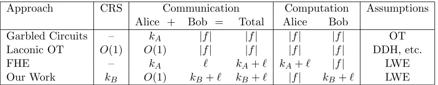
linear dependence on the output size |y|is inherent for any (semi-malicious) secure protocol, as shown in [HW15] but it remains an interesting open problem to get rid of the dependence on the circuit depth d. We summarize the comparison of different approaches in Figure 1.
Our protocol using LFE is extremely simple: Alice sends a digest for the functionf(xA,·) in the first
round and Bob uses the digest to encrypt xB in the second round. To get security for Alice, we use a
function-hiding LFE scheme and we even ensure that Alice’s security holds statistically. The above gives
4
Approach CRS Communication Computation Assumptions
Alice + Bob = Total Alice Bob
Garbled Circuits – kA |f| |f| |f| |f| OT
Laconic OT O(1) O(1) |f| |f| |f| |f| DDH, etc.
FHE – kA ` kA+` kA+` |f| LWE
Our Work kB O(1) kB+` kB+` |f| kB+` LWE
Figure 1: Summary of semi-honest 2-round 2PC where Alice holdsxA∈ {0,1}kA, Bob holdsxB∈ {0,1}kB,
and Alice learns y =f(xA, xB) ∈ {0,1}`. We suppress multiplicative factors that are polynomial in the
security parameter λ or, for the last row, the circuit depthd.
us a 2PC with semi-honest security. We can think of this as a protocol in the CRS model, or we can even allow Alice to choose the CRS on her own and send it in the first round to get a protocol in the plain model. If we think of it as a protocol in the CRS model, we even get “semi-malicious” security where corrupted parties follow the protocol but can use maliciously chosen randomness. To get fully malicious security we would need to additionally rely on succinct non-interactive zero-knowledge arguments of knowledge (ZK-SNARKs) [Mic94, Gro10, BCCT13, BCI+13, GGPR13] and have Alice prove that she
computed the digest correctly.
MPC with Small Online Computation. As our second application, we construct an MPC protocol that allows N parties to securely evaluate some functionf(x1, ..., xN) over their respective inputs, where
the total amount of computation performed by the parties during the protocol execution is smaller than that of evaluating the function itself! Of course, the work of the computation must be performed at some point, even if we didn’t care about security. In our case, the MPC protocol requires each party to individually pre-process the function f step before the protocol starts and to post-process the protocol transcript and recover the output after the protocol ends, where the computational complexity of these steps can exceed the circuit size off. The pre-processing step is deterministic and can be performed once per function being evaluated and reused across many executions. However, the main novelty of our MPC is that the total computation performed by the partiesonline, from the time they send the first protocol message and until they receive the last protocol message, is much smaller than the circuit size off. This also implies a correspondingly small communication complexity of the protocol.
(We note there are prior MPC protocols that have a separate “offline” phase, which occurs before the inputs of the computation are known, and an “online” phase which occurs after the inputs are known and where the online phase is very efficient. However, in these schemes the term “offline” is a misnomer since the offline phase involves running a protocol and interacting with the other parties. For example, the parties may run an MPC protocol to compute a garbled circuit for the functionf in the offline phase and then, once their inputs are known, they run another much more efficient MPC protocol to compute the garbled input for the garbled circuit. In contrast, ours is the first MPC that has a truly offline pre-processing and post-processing phase, where the parties do not interact with each other, while the computational complexity of the entire online phase that involves interaction is smaller than the circuit size.)
Our MPC construction uses an LFE scheme and proceeds as follows:
Pre-processing (offline). Each party individually pre-processes the circuitfby locally computingdigestf =
Compress(f). We rely on an LFE scheme with deterministic compression so all parties compute the same digest. This step can be performed once and can be reused across many executions.
Actual protocol (online). The actual protocol execution between the N parties holding inputs xi just
invokes a generic MPC protocol to compute an LFE ciphertext ct ← Enc(digestf,(x1, . . . , xN))
Post-processing (offline). After the protocol finishes, each party individually does a post-processing step in which it runs the LFE decryption algorithm onct to recover the output f(x1, . . . , xN).
The computational complexity of the pre-processing and post-processing steps is|f|·poly(λ, d), wheredis the depth of the circuit f. The computational complexity of each party in the online protocol execution and the total communication complexity are only poly(λ, d, k, `, N), where k is the input size of each party and ` is the output size and N is the number of parties. In particular, the communication and computational complexity of the online phase can be much smaller than the circuit size of f. We inherit semi-honest or fully-malicious security depending on the MPC used in online phase. We think of the above protocol as being in the CRS model. However, in the case of semi-honest security, we can also think of it as a protocol in the plain model by having a single designated party (e.g., party 1) choose the CRS for the LFE and compute the digest digestf (no other parties do any pre-processing) and use these as its inputs to the MPC protocol executed in the online phase.
By taking our scheme from the previous paragraph and using a 2-round MPC [MW16, PS16, BP16, GS17, BL18, GS18] in the online phase (without any additional efficiency constraints), we get a 2-round MPC where the total computation performed by each party (including pre-processing and post-processing) is|f| ·poly(λ, d) +poly(λ, k, `, d, N) and the total communication ispoly(λ, k, `, d, N). In all prior 2-round MPC protocols withN parties (even with semi-honest security, even in the CRS model), the computation performed by each party is at least|f| ·N2. Therefore our result gives improved computational efficiency
for 2-round MPC even if we did not distinguish between online and offline work. In the case of semi-honest security, if we use a 2-round MPC in the plain model [GS17, BL18, GS18] in the online phase we get a 2-round MPC in the plain-model with the above efficiency. In particular, we get a semi-honest 2-round MPC in the plain model with communication which is smaller than the circuit size, matching the recent work of Ananth et al. [ABJ+18] which previously got such result using functional-encryption combiners.
1.3 Our Techniques
Our construction of LFE relies on an adaptation of techniques developed in the context of attribute-based and functional encryption [BGG+14, GKP+13]. The construction proceeds in two steps. We start by considering LFE for a restricted class of functionalities, which we call attribute-based LFE (AB-LFE) in analogy to attribute-based encryption (ABE). In an AB-LFE, Alice computes a digest digestf for a function f. Bob computes a ciphertext Enc(digestf, x, µ) with an attributex and a messageµ such that Alice recovers µ if f(x) = 0 and otherwise doesn’t learn anything about µ. (For technical reasons, it will be easier to use the semantics where 0 denotes “qualified to decrypt” and 1 denotes “unqualified to decrypt”.) However, the attribute x is always revealed to Alice. We can think of AB-LFE as an LFE for the “conditional disclosure functionality” CDF[f](x, µ), which outputs (x, µ) if f(x) = 0 and (x,⊥) otherwise. As our first step, we construct AB-LFE under the LWE assumption. As our second step, we show how to generically compile any AB-LFE into an LFE by additionally relying on fully homomorphic encryption.
We rely on two algorithms EvalPK,EvalCT that were defined by [BGG+14]. Let G ∈
Zn×mq be
a fixed “gadget matrix” from [MP12]. Let Ai ∈ Zn×mq be arbitrary matrices, bi ∈ Zmq be vectors,
f :{0,1}k→ {0,1}be some circuit andx∈ {0,1}k be an input.
• EvalPK(f,{Ai}i∈[k]) outputs a matrix Af ∈Zn×mq .
• EvalCT(f,{Ai}i∈[k],{bi}i∈[k], x) outputs a vector bf ∈Znq.
These algorithms are deterministic and have the property that:
if {bi =s>(Ai−xiG) +ei}i∈[k] then bf =s>(Af −f(x)G) +e∗ (1)
where ei and e∗ are some “small” errors. Our basic AB-LFE scheme works as follows.
• The CRS consists of uniformly random matricesA1, . . . ,Ak withAi ∈Zn×mq .
• To compress a circuitf : {0,1}k→ {0,1}we set the digest to bedigestf =Af =EvalPK(f,{Ai}i∈[k]).
• The encryption algorithm Enc(digestf, x, µ) encrypts a message µ ∈ {0,1} with respect to an at-tribute x ∈ {0,1}k under a digest digestf = Af. It chooses a random LWE secret s ← Znq and
computes LWE samplesbi =s>(Ai−xiG) +ei. It also chooses a random “short” vectortand sets d=Af ·t. Lastly it setsβ =hs,di+e0+µ· bq/2e and outputs the ciphertext ct= ({bi}, β,t, x).
• The decryption algorithm computes bf =EvalCT(f,{Ai}i∈[k],{bi}i∈[k], x). By (1), we have bf = s>(Af −f(x)G) + e∗. If f(x) = 0 then this allows us to recover the message by computing
β− hbf,ti ≈µ· bq/2e.
To prove security, we assume that f(x) = 1 and need to show that the ciphertext doesn’t reveal anything about the encrypted message µ. We can rely on the LWE assumption with a uniformly random secret s and coefficient (Ai −xiG) to argue that the samples bi are indistinguishable from uniform.
However, to argue that β is also indistinguishable from uniform is slightly more complex. Firstly, we note that by (1), we have β ≈ hbf,ti+s>Gt+e0 +µ· bq/2e. Secondly, if we set u = Gt, then u is
uniformly random and t ← G−1(u) can be efficiently sampled from u, so we can efficiently sample β
given u,hs,ui+e0+µ· bq/2e. Therefore, when we use the LWE assumption, we also get one additional sample with the coefficients u which we use to argue that β is indistinguishable from uniform. There is some subtlety in ensuring that the noise distribution in β is correct and we solve this using the standard “noise smudging” technique.
Adaptively Secure AB-LFE from Adaptive LWE. The above proof shows selective security, where the adversary chooses the attributex ahead of time before seeing the CRS, but breaks down in the case of adaptive security. The issue is that, if the attributex is chosen adaptively after the adversary sees the CRS = {Ai}, then we can no longer argue that the LWE coefficients (Ai−xiG) are uniformly random.
However, the adversary has extremely limited ability to manipulate the coefficients. We formulate a new but natural “adaptive LWE” assumption where the adversary is first given matrices {Ai}i∈[k], then
adaptively chooses a value x∈ {0,1}k, and has to distinguish between LWE sampless>(Ai−xiG) +ei
Another interesting question is whether the adaptive LWE assumption could be useful in proving adaptive security in other contexts, most notably for attribute-based encryption (ABE) of Boneh et al. [BGG+14]. As far as we can tell, this does not appear to be the case, and the reason that we are able to prove adaptive security of AB-LFE under adaptive LWE is that our proof differs significantly from that of the Boneh et al. ABE and does not rely on embedding lattice trapdoors in the CRS. Nevertheless, we leave this as an interesting possibility for future work.
Second Step: From AB-LFE to LFE. As our second step, we show how to generically compile AB-LFE to LFE using fully-homomorphic encryption (FHE). This compiler is essentially identical to that of Goldwassser et al. [GKP+13], which showed how to compile attribute-based encryption (ABE) to (single key) functional encryption (FE). In addition to FHE, the compiler relies on garbled circuits which can be constructed from one-way functions.
The high level idea is that, in the LFE scheme, the encryptor Bob first uses an FHE to encrypt his input x, resulting in an FHE ciphertext xb. He then constructs a garbled circuit Cb which has the FHE secret key hard-coded inside of it and performs an FHE decryption. Lastly, he uses an AB-LFE scheme to encrypt all of the labels of the input wires of the garbled circuit with respect to the attribute
b
x in such a way that Alice recovers exactly the garbled labels that correspond to the homomorphically evaluated ciphertextfd(x) =FHE.Eval(f,
b
x). Bob sends bx,Cb and the AB-LFE ciphertexts to Alice as his LFE ciphertext.
Optimizing for Long Output and Final Parameters. The above ideas, combined together, give an LFE scheme for circuits f : {0,1}k → {0,1} with 1-bit output and depth d, where the digest is of size poly(λ, d) and the encryption run-time and ciphertext size is k·poly(λ, d). The compression and decryption run-time is |f| ·poly(λ, d).
A naive way to get an LFE for circuitsf : {0,1}k → {0,1}` with`-bit output is to invoke a separate LFE for each output bit. This would blow up all of the efficiency measures by a multiplicative factor of
`. It turns out that we can do better. We do so by first constructing a “multi-bit output AB-LFE” that allows Alice to compute a digest digestf for a circuit f : {0,1}k → {0,1}` with `-bit output and for Bob to create a single ciphertext with an attribute x and messages µ1, . . . , µ` such that Alice recovers
µi if and only if the i’th output bit of f(x) is 0. We show how to modify our LWE based AB-LFE
construction to get a “multi-bit output AB-LFE” where the encryption run-time and the ciphertext size is (k+`)·poly(λ, d) and the compression/decryption run-times remains|f|·poly(λ, d). However, the digest size in this construction grows by a factor of `to`·poly(λ, d). We then show how to compress the digest further to just poly(λ) independent of`, d. Essentially, instead of using the original AB-LFE digest as is, we employ an additional layer of laconic OT (LOT) and give out an LOT digest of the AB-LFE digest. The encryptor creates a garbled version of the underlying AB-LFE encryption algorithm and encrypts the labels for the garbled circuit under LOT.
Combining all of the above we get an LFE scheme where the size of the CRS is k·poly(λ, d), the size of the digest is poly(λ), the run-time of the encryption algorithm and the size of the ciphertext are
e
O(k+`)·poly(λ, d) and the run-time of the compression and the decryption algorithms isOe(|f|)·poly(λ, d).
2
Preliminaries
2.1 Notations
We will denote by λ the security parameter. The notation negl(λ) denotes any function f such that
f(λ) = λ−ω(1), and poly(λ) denotes any function f such that f(λ) = O(λc) for some c > 0. For a probabilistic algorithmalg(inputs), we might explicit the randomness it uses by writtingalg(inputs;coins). We will denote vectors by bold lower case letters (e.g. a) and matrices by bold upper cases letters (e.g.
A). We will denote by a> and A> the transposes of a and A, respectively. We will denote by bxe the nearest integer to x, rounding towards 0 for half-integers. If x is a vector, bxe will denote the rounded value applied component-wise.
We define the statistical distance between two random variables X and Y over some domain Ω as: SD(X, Y) = 12P
w∈Ω|X(w)−Y(w)|. We say that two ensembles of random variables X = {Xλ},
Y ={Yλ} arestatistically indistinguishable, denoted X s
≈Y, ifSD(Xλ, Yλ)≤negl(λ).
We say that two ensembles of random variables X = {Xλ}, and Y = {Yλ} are
computation-ally indistinguishable, denoted X ≈c Y, if, for all (non-uniform) PPT distinguishers Adv, we have
|Pr[Adv(Xλ) = 1]−Pr[Adv(Yλ) = 1]| ≤negl(λ).
2.2 Learning With Errors
Definition 2.1 (B-bounded distribution). We say that a distribution χ over Z is B-bounded if
Pr[χ∈[−B, B] ] = 1.
We recall the definition of the (decision)Learning with Errorsproblem, introduced by Regev ([Reg05]).
Definition 2.2 ((Decision) Learning with Errors ([Reg05])). Let n =n(λ) and q =q(λ) be integer pa-rameters and χ=χ(λ) be a distribution overZ. The Learning with Errors (LWE) assumptionLW En,q,χ
states that for all polynomials m=poly(λ) the following distributions are computationally indistinguish-able:
(A,s>A+e)≈c (A,u)
where A←Zn×mq ,s←Znq,e←χm,u←Zmq .
Just like many prior works, we rely on LWE security with the following range of parameters. We assume that for any polynomial p = p(λ) = poly(λ) there exists some polynomial n =n(λ) = poly(λ), someq=q(λ) = 2poly(λ) and someB =B(λ)-bounded distributionχ=χ(λ) such thatq/B ≥2p and the
LW En,q,χ assumption holds. Throughout the paper, theLWE assumption without further specification
refers to the above parameters. The sub-exponentially secure LWE assumption further assumes that
LW En,q,χ with the above parameters is sub-exponentially secure, meaning that there exists someε >0
such that the distinguishing advantage of any polynomial-time distinguisher is 2−λε.
The works of [Reg05, Pei09] showed that the (sub-exponentially secure) LWE assumption with the above parameters follows from the worst-case (sub-exponential) quantum hardness SIVP and classical hardness of GapSVP with sub-exponential approximation factors.
2.3 Lattice tools
Noise smudging. We will use the following fact.
Lemma 2.3 (Smudging Lemma (e.g., [AJL+12])). Let B = B(λ), B0 = B0(λ) ∈ Z be parameters and and let e1 ∈[−B, B] be an arbitrary value. Let e2 ← [B0, B0]be chosen uniformly at random. Then the
Gadget Matrix [MP12]. For an integerq ≥2, define: g= (1,2,·,2dlogqe−1)∈Z1×dlogq qe.The Gadget
Matrix G is defined as G =g⊗In ∈ Zn×mq where n∈N and m =ndlogqe. There exists an efficiently
computable deterministic functionG−1 : Znq → {0,1}msuch for allu∈Znq we haveG·G−1(u) =u. We
let G−1($) denote the distribution obtained by sampling u ← Znq uniformly at random and outputting t=G−1(u).
Lattice Evolution. We rely on the following algorithms introduced in [BGG+14].
Claim 2.4 ([BGG+14]). Let n∈N andm=ndlogqe. There exists two deterministic algorithms EvalPK
and EvalCT with the following syntax:
• EvalPK(C,A1, . . . ,Ak) takes as input a circuitC : {0,1}k→ {0,1} and matricesAi∈Zn×mq , and
outputs a matrix AC ∈Zn×mq ;
• EvalCT(C,A1, . . . ,Ak,b1, . . .bk, x) takes as input a circuit C : {0,1}k → {0,1}, matrices Ai ∈
Zn×mq , vectors bi ∈Zmq and an input x∈ {0,1}k, and outputs a vector bC ∈Zmq ;
such that if there exists some s∈Zn
q such that:
∀i≤k, bi=s>(Ai−xiG) +ei withkeik∞≤B,
then
bC =s>(AC−C(x)G) +eC where keCk∞≤(m+ 1)d·B.
Furthermore, the run-time of EvalPK,EvalCT is |C| ·poly(n,logq).
We can extend the above algorithms to support circuitsC : {0,1}k→ {0,1}` with multi-bit output. In this case, we have that:
• EvalPK(C,A1, . . . ,Ak) outputs ` matrices{ACj}j≤` ∈(Z
n×m q )`;
• EvalCT(C,A1, . . . ,Ak,b1, . . .bk, x) outputs `vectors {bCj}j≤`∈(Z
m q )`.
The output is identical to having run EvalPK,EvalCT separately for each output bit of C. However, by processing the entire circuit in one shot (rather than looking at each output bit separately), we ensure that the run-time of EvalPK,EvalCTremains|C| ·poly(n,logq) instead of |C| ·`·poly(n,logq).
2.4 Fully Homomorphic Encryption
A leveled Fully Homomorphic Encryption scheme (FHE) is a set of algorithms (FHE.KeyGen,FHE.Enc,
FHE.Dec,FHE.Eval) satisfying the following properties:
• Security: (FHE.KeyGen,FHE.Enc,FHE.Dec) is a semantically secure encryption scheme;
• Perfect correctness: For allλ, all C:{0,1}k→ {0,1}` of depthdand x∈ {0,1}k:
PrhFHE.Dechsk(FHE.Eval(C,FHE.Enchpk(x))) =C(x) | (hpk,hsk)←FHE.KeyGen(1λ,1d) i
= 1;
• Compactness: If C : {0,1}k → {0,1}` is a circuit of depth d, then the output length of FHE.Eval(C,·) should be`·poly(λ, d).
• Efficiency: IfC:{0,1}k→ {0,1}`is a circuit of depthd, thenFHE.Eval(C,·), which takes as input
a ciphertext ct, and outputs FHE.Eval(C,ct) can be computed by a circuit of depth d·polylog(λ) and size |C| ·poly(λ, d).
2.5 Garbled Circuits
We define here garbled circuits, originally introduced by Yao ([Yao82]), and there are now many variants in the literature ([BHR12]). The following formalization is heavily inspired by the one used in [GKP+13].
A Garbling Scheme is a set of algorithms (GC.Garble,GC.Eval) such that:
• GC.Garble(1λ, C) takes as input the security parameter λ, a circuit C : {0,1}k → {0,1}`, and
outputs a garbled circuit Γ and a set of labels {L0i, L1i}i≤k.
• GC.Eval(Γ,{Li}i≤k) takes as input a garbled circuit and a subset of labels, and outputs a value
y∈ {0,1}`.
• AlgorithmsGC.Garbleand GC.Eval satisfy the following properties:
Correctness. We have for all circuitsC:{0,1}k → {0,1}` and for allx∈ {0,1}k:
Pr[C(x) =y | (Γ,{L0i, L1i}i≤k)←GC.Garble(1λ, C), y←GC.Eval(Γ,{Lxii}i≤k) ] = 1,
where xi denotes theith bit ofx.
Circuit and Input privacy. Define the two following experiments:
expRealGC (1λ) : expIdealGC (1λ) :
1. (x, C)←Adv(1λ) 1. (x, C)←Adv(1λ)
2. (Γ,{L0i, L1i}i≤k)←GC.Garble(1λ, C) 2. (˜Γ,{L˜i}i≤k)←SimGC(1λ,|C|,|x|, C(x))
3. b∈ {0,1} ←Adv(Γ,{Lxi
i }i≤k) 3. b∈ {0,1} ←Adv(˜Γ,{L˜i}i≤k)
4. Output b. 4. Outputb.
We say that (GC.Garble,GC.Eval) is circuit and input private if there exists a PPT simulator SimGC
such that for all stateful PPT adversary Adv, we have:
Pr
h
expRealGC (1λ) = 1
i
−PrhexpIdealGC (1λ)
i
≤negl(λ).
Efficiency. For any circuit C, and (Γ,{L0
i, L1i}i≤k)← GC.Garble(1λ, C), we have the following
proper-ties:
• GC.Garble(1λ, C) has complexity|C| ·poly(λ);
• GC.Eval(Γ,·) has complexity|C| ·poly(λ);
• Γ is of size |C| ·poly(λ);
• Lbi is of sizepoly(λ) for alli≤kand b∈ {0,1}.
2.6 Entropy and Extractors
The min-entropy of a random variableX, is defined asH∞(X) =−log(maxxPr[X=x]). The(average)
conditional min-entropy [DORS08] of a random variableX conditioned on Y, is defined as H∞(X|Y) = −log(EymaxxPr[X=x|Y =y]).
Lemma 2.5 ([DORS08]). If X, Y, Z are jointly distributed random variables and the support of Y is Y
We say that Ext : X × S → Y is a (k, )-extractor, if for all joint distribution (X, Z) where X is supported overX and H∞(X|Z)≥k, we have:
SD( (Ext(X;S), Z, S),(Y, Z, S) )≤,
where S is uniform over S andY is uniform over Y.
The following lemma states that universal hash functions are good extractors:
Lemma 2.6 (Leftover Hash Lemma [ILL89, DORS08]). Let H={Hseed:X → Y}seed∈S be a universal
hash function family. Then Ext(x;seed) =Hseed(x) is a (k, ε)-extractor for k= log(|Y|) + 2 log(1/ε).
3
Definition of LFE
In this section, we define our notion of laconic function evaluation (LFE) for a class of circuits C. We assume that the class C associates every circuit C ∈ C with some circuit parameters C.params. For our default notion of LFE throughout this paper, unless specified otherwise, we will consider Cto be the class of all circuits withC.params= (1k,1d) consisting of the input size k and the depthdof the circuit.
Definition 3.1 (LFE). A laconic function evaluation (LFE) scheme for a class of circuitsC consists of four algorithms crsGen , Compress , Enc and Dec.
• crsGen(1λ,params) takes as input the security parameter 1λ and circuit parameters params and outputs a uniformly random common random stringcrs of appropriate length.5
• Compress(crs, C)is a deterministic algorithm that takes as input the common random stringcrs and a circuit C∈ C and outputs a digest digestC.
• Enc(crs,digestC, x) takes as input the common random string crs, a digest digestC and a message x
and outputs a ciphertext ct.
• Dec(crs, C,ct) takes as input the common random string crs, a circuit C ∈ C, and a ciphertext ct
and outputs a message y.
We require the following properties from those algorithms:
Correctness: We require that for all λ,params andC ∈ C withC.params=params:
Pr
y=C(x)
crs ←crsGen(1λ,params)
digestC =Compress(crs, C)
ct ←Enc(crs,digestC, x)
y ←Dec(crs, C,ct)
= 1.
Security: We require that there exists a PPT simulator Sim such that for all stateful PPT adversary
Adv, we have:
Pr
h
expRealLF E(1λ) = 1
i
−PrhexpIdealLF E(1λ)
i
≤negl(λ) for the experiments expRealLF E(1λ) and expIdealLF E(1λ) defined below:
5
expRealLF E(1λ) : expIdealLF E(1λ) :
0. params←Adv(1λ) 0. params←Adv(1λ) 1. crs←crsGen(1λ,params) 1. crs←crsGen(1λ,params) 2. x∗, C ←Adv(crs): 2. x∗, C ←Adv(crs):
C∈ C , C.params=params C∈ C , C.params=params
3. digestC =Compress(crs, C) 3. digestC =Compress(crs, C) 4. ct←Enc(crs,digestC, x∗) 4. ct←Sim(crs, C,digestC, C(x∗)) 5. Output Adv(ct) 5. Output Adv(ct)
We refer to the above as adaptive security. We also define a weaker version of selective security where the above experiments are modified so that Adv has to choose x∗ at the very beginning of the experiment in step 0, before seeing crs (but can still choose C adaptively).
Composability. Note that, in our security definition, the simulator is given a correctly generatedcrs
as an input rather than being able to sample it itself. This guarantees composability. Given several ciphertexts cti encrypting various inputs xi under the same or different digests digestCj, all using the same crs, we can simulate all of them simultaneously and security follows via a simple hybrid argument where we switch them from real to simulated one by one.
Efficiency. The above definition does not directly impose any efficiency restrictions and can therefore be satisfied trivially by setting digestC =C and Enc(digestC, x) =C(x). The main goal will be to ensure
that the LFE scheme is laconic, meaning that the size of crs,digestC,ct and the run-time of Enc should all be as small as possible and certainly smaller than the circuit size of C. We will discuss the efficiency of our constructions as we present them.
4
Construction of LFE from LWE
In this section, we construct LFE for all circuits under the LWE assumption with subexponential modulus-to-noise ratio. As a stepping stone to build LFE, we consider LFE for a restricted class of functionalities, which we call attribute-based LFE (AB-LFE) in analogy to attribute-based encryption (ABE).
Definition of AB-LFE. Let C :{0,1}k → {0,1} be a circuit. We define the Conditional Disclosure
Functionality (CDF) of C as the function
CDF[C](x, µ) = (
(x, µ) ifC(x) = 0; (x,⊥) ifC(x) = 1,
where x∈ {0,1}k, and µ∈ {0,1}.
We also generalize this tomulti-bit outputs. For a circuitC :{0,1}k→ {0,1}`
we define
CDF[C](x,(µ1, . . . , µ`)) = (x,(˜µ1, . . . ,µ˜`)) where
( ˜
µj =µj ifCj(x) = 0;
˜
µj =⊥ifCj(x) = 1.
,
where x∈ {0,1}k, µj ∈ {0,1}w and Cj(x) denotes thej’th output bit ofC(x).
We will consider canonical descriptions ofCDF[C] such that one can efficiently recoverCgivenCDF[C]. To simplify notation for AB-LFE we will give the algorithms of the AB-LFE the circuit C as input rather than CDF[C]. E.g., we will write digestC ← Compress(crs, C) instead of the more cumbersome
digestCDF[C]←Compress(crs,CDF[C]).
Outline. In Section 4.1, we build an AB-LFE for circuitsCwith single-bit output. We then present an optimized construction that supports circuits with multi-bit output in Section 4.2. We discuss adaptive security for our constructions in Section 4.3. In Section 4.4, we give a generic transformation from AB-LFE to LFE (assuming FHE).
4.1 Basic AB-LFE from LWE
We first present our simplest construction of an AB-LFE from LWE for the case of a single bit output.
Parameters. We fix integer parametersn, m, q, B, B0∈Zand aB-bounded distributionχoverZ, all of
which are functions of λ, d. In particular, we setm=ndlogqeand the choice ofn, q, χ, B comes from the LWE assumption (see Section 2.2) subject to n=poly(λ, d), q= 2poly(λ,d),and q/B = 8·(m+ 1)d+1·2λ. We set B0 =B·(m+ 1)d+1·2λ.
Construction. We define the procedurescrsGen,Compress ,Enc and Dec as follows.
• crsGen(1λ,params= (1k,1d)): Pick krandom matrices Ai ←Zn×mq and set:
crs= (A1, . . . ,Ak).
• Compress(crs, C): Output:
digestC =AC =EvalPK(C,{Ai}i≤k),
where EvalPKis defined in Section 2.3.
• Enc(crs,AC,(x, µ)): Pick a random s←Znq,ei←χm fori≤k, and compute:
bi=s>(Ai−xiG) +e>i , i≤k.
Sample t←G−1($),6 set d=AC·t, and compute
β =s>d+ee+µ· bq/2e,
where ee←[−B0, B0]. Output:
ct= ({bi}i≤k, β,t, x).
• Dec(crs, C,ct): IfC(x) = 1 output⊥. Else compute:
e
b=EvalCT(C,{Ai}i≤k,{bi}i≤k, x),
where EvalCTis defined in Section 2.3. Outputb(β−eb>t)/qe.
6RecallG−1($) denotes the distribution of samplingu←
Proof overview. The key observation underlying both correctness and security is that for honestly generated ciphertexts, we have:
e
b≈s>[AC−C(x)G]
and therefore
β−eb·t≈C(x)·s>G·t. (2)
In the proof, we will use the above equation to simulate β aseb·t+C(x)·s>G·t.
Claim 4.2 (Correctness). The construction is correct.
Proof. AssumeC(x) = 0. Then, by correctness of EvalCT, we have:
e
b=EvalCT(C,{Ai}i≤k,{bi}i≤k, x) =s>[AC−C(x)G] +e>C =s >
AC+e>C,
with keCk∞≤(m+ 1)d·B. Thereforebe>t=s>d+e>C·t and
β−be>t= (s>d+ee+µ· bq/2e)−(s>d+e>C ·t) =µ· bq/2e+ee−e>C·t
where |ee−e>C·t| ≤(m+ 1)d+1·B+B0<2B·(m+ 1)d+1·2λ< q/4.
Claim 4.3 (Security). The construction is selectively secure under the LWE assumption LWEn,q,χ.
Proof. Note that the simulator is given C, x∗ and CDF[C](x∗, µ∗) as input. In particular, if C(x∗) = 0 then the simulator is given (x∗, µ∗) in full and can therefore create the ciphertext honestly as in the Real experiment. So without loss of generality, we can concentrate on the caseC(x∗) = 1. Define the following simulator:
• Sim(crs,digestC, C, x∗): pickbi←Zqm fori≤k, pick β←Zq, and t←G−1($). Output:
ct= ({bi}i≤k, β,t, x∗).
We prove that the experimentsexpRealLF E(1λ) andexpIdealLF E(1λ) from Definition 3.1 are computationally
indistinguishable via a sequence of hybrids.
Hybrid 0. This is the real experiment expRealLF E(1λ).
Hybrid 1. Here the way β is computed is modified. After computingbi =s>(Ai−x∗iG) +e>i and
sampling t ← G−1($), compute eb = EvalCT(C,{Ai}i≤k,{bi}i≤k, x∗) and α = s>Gt+e0 ∈ Zq, where
e0 ←χ. Set
β=eb·t+α+ e
e+µ· bq/2e,
where ee←[−B
0, B0].
By correctness ofEvalCTand the fact that C(x∗) = 1, we haveeb=s>(AC −G) +e>C, so that
e
b·t+α=s>AC·t+e>C ·t+e0=s>d+e>C·t+e0
and therefore, in Hybrid 1, we have
β =s>d+µ∗· bq/2e+ee+ (e
>
C·t+e0).
Hybrid 2. In this hybrid we pick α and {bi}i≤k uniformly at random. We still sample t←G−1($)
and compute eb=EvalCT(C,{Ai}i≤k,{bi}i≤k, x) and β =be·t+α+ee+µ∗· bq/2e as previously.
We show that Hybrid 1 and Hybrid 2 are computationally indistinguishable under LWEn,q,χ. More
precisely, the reduction receives x∗ from the adversary and gets LWE challenges (u, α) and (Mi,bi)i≤k,
where u ← Znq,Mi ← Zn×mq . It sets crs ={Ai =Mi+x∗iG}i≤k, and t =G−1(u), and computes β as
previously. Then, if α and {bi} are distributed as LWE samples, then the view of the adversary is as in
Hybrid 1; if they are uniform, then its view is distributed as in Hybrid 2.
Note that Hybrid 2 corresponds toexpIdealLF E(1λ) with the simulatorSimdefined above since the values
β and {bi}i≤k in Hybrid 2 are uniformly random.
Comparison with the ABE from [BGG+14]. Our construction is very reminiscent of the ABE from [BGG+14]. In their ABE scheme, there is an additional matrixA
0, and the relation d=AC·t is
replaced withd= [A0|AC]·t. The quantitiesA0,dare part of the master public key andtis the secret
key corresponding to the circuit C. The ABE security proof needs to take into account an adversary that sees many such t’s with respect to the samed.
There are several key differences between our AB-LFE and the prior ABE scheme. A crucial distinction is that our Encryption algorithm takesAC as input, which allows it to samplet and then setd=AC·t.
The value t is a part of our ciphertext. In [BGG+14], the analogous operation is performed by having
a trapdoor for A0 as a master secret key of the ABE and using this trapdoor to sample t that satisfies d = [A0 |AC]·t during key generation and including it as part of the secret key for the circuit C. The
proof of security for the ABE scheme is also significantly more complex and involves carefully “puncturing” the public matrices in Ai in thecrs so as to be able to provide secret keys for circuits C if and only if
C(x) = 1. The fact that we don’t need any trapdoors for our construction essentially paves our way to a much simpler proof.
Message-adaptivity. To argue indistinguishability between Hybrids 1 and 2 from LWE, the reduction needs to know the challenge attributex∗ ahead of time to create thecrs using its LWE challenges, which makes the construction selectively secure. However, it doesn’t need to know the messageµ∗at that point. In particular, our construction is “message-adaptive”, where the adversary has to choose the challenge attribute x∗ before seeing the crs, but can choose the challenge message µ∗ after seeing the crs.
Efficiency. For circuits with input lengthk, 1-bit output and depthdthe above construction of AB-LFE from LWE has the following parameters.
• The crs is of sizek·poly(λ, d). The digest is of sizepoly(λ, d).
• The run-time of the encryption algorithm and the size of the ciphertext are k·poly(λ, d).
• The run-time of the compression and the decryption algorithms is |C| ·poly(λ, d).
4.2 Improved AB-LFE for Multi-Bit Output
We extend the construction to AB-LFE with multi-bit output. Recall that in this case the encryption algorithm takes as input (x,µ1, . . . ,µ`) and the decryption algorithm recoversµj for allj such that the
j’th bit of C(x) is 0. We use the notation Cj(x) to denote the j’th bit of C(x). As another difference
from the single-bit case, we now also allow the messages µj ∈ {0,1}w to be multi-bit messages rather than a single bit.
across all of them). In that case, all efficiency measures blow up by a multiplicative factor of `: the size of the ciphertext would be `·k·poly(λ, d), the size of the digest would be`·poly(λ, d) and the run-time of the compression/decryption algorithms would be `· |C| ·poly(λ, d). We show that we can do better in two steps. First, we show how to compress the ciphertext size to only (`+k)·poly(λ, d) instead of
`·k·poly(λ, d) and the encryption/decryption run-time to |C| ·poly(λ, d) instead of `· |C| ·poly(λ, d). In essence, we show how to reuse the “x part” of the ciphertext across all ` copies. Second, we show how to also compress the digest from `·poly(λ, d) to just poly(λ) without blowing up any of the other parameters.
4.2.1 Compressing the Ciphertext
Construction. We fix the parametersn, m, q, B, B0, χas in the single bit case.
• crsGen(1λ,params= (1k,1d)): Pick krandom matrices Ai ←Zn×mq and set:
crs= (A1, . . . ,Ak).
• Compress(crs, C): LetC : {0,1}k→ {0,1}`. Output:
digestC ={ACj}j≤` =EvalPK(C,{Ai}i≤k),
where EvalPKover multi-bit output circuits is defined in Section 2.3.
• Enc(crs,{ACj}j≤`,(x,{µj}j≤`)): Let µj ∈ {0,1} w
forj≤`. Pick s←Zn
q,ei←χm fori≤k, and compute:
bi=s>(Ai−xiG) +e>i , i≤k,
For j≤`, sample Tj ←(G−1($))w ∈Zm×wq , setDj =ACj·Tj, and compute for all j≤`
βj =s>Dj+ee
>
j +µj · bq/2e ∈Z1×wq ,
whereeej ←[−B, B]w. Output:
ct= ({bi}i≤k,{βj}j≤`,{Tj}j≤`, x).
• Dec(crs, C,ct): Compute
n e
bj
o
j≤`=EvalCT(C,{Ai}i≤k,{bi}i≤k, x).
For allj ≤`, ifCj(x) = 1 setµj =⊥; else setµj =b(βj−bejTj)/qe. Output (µ1, . . .µ`).
Correctness follows directly by the same argument as for Claim 4.2. For security, we want to ensure that µj is hidden whenever Cj(x∗) = 1. However, there are some differences from the single output bit
case here since we may have Cj(x∗) = 1 for some j and Cj(x∗) = 0 for others.
Claim 4.4 (Security). The above construction is selectively secure under the LWE assumption LWEn,q,χ.
Proof. Note that the simulator is givenCDF[C](x∗,(µ1, . . . ,µ`)) as input. Denote byI the set of indices
j ≤`such thatCj(x∗) = 0. For allj∈I, the simulator is givenµj while for all otherj6∈I the simulator
• Sim(crs,digestC, C,CDF[C](x∗,(µ1, . . . ,µ`))): Pick bi ←Zmq for all i≤k andTj ←(G−1($))w for
all j≤`, and compute: n
e
bj
o
j≤` =EvalCT(C,{Ai}i≤k,{bi}i≤k, x ∗).
– For allj ∈I compute:
βj =ebj·Tj+ e
e>j +µj· bq/2e,
whereeej ←[−B0, B0]w.
– For allj /∈I pick βj ←Zq uniformly at random.
Output:
ct= ({bi}i≤k,{βj}j≤`,{Tj}j≤`, x∗).
The hybrids follow closely the ones of the proof for the 1-bit version in Section 4.1. There are a few differences:
Hybrid 1. The way the vectorsβj are generated now depends onCj(x∗).
We compute bi =s>(Ai−x∗iG) +e>i fori≤k (where ei ←χm), and pickTj ← (G−1($))w for all
j ≤`, and setnbej o
j≤`=EvalCT(C,{Ai}i≤k,{bi}i≤k, x
∗). Then, for allj≤`:
• If j∈I (i.e. Cj(x∗) = 0), we directly setβj =ebj·Tj+ee>j +µj· bq/2e, whereeej ←[−B0, B0]w.
• If j /∈ I (i.e. Cj(x∗) = 1) we compute αj = s>GTj +e>0,j, where e0,j ← χw, and set βj =
e
bj·Tj+αj+ee
>
j +µj· bq/2e, whereeej ←[−B
0, B0]w.
Indistinguishability from the Hybrid 0 follows by the same argument as in the previous proof, asbej =
s>[ACj−Cj(x
∗)G] +e>
Cj by correctness of EvalCT, whereCj(x
∗) = 0 if j∈I and C
j(x∗) = 1 otherwise.
Lemma 2.3 then ensures that the distributions of ee>j (noise of βj in Hybrid 0), and ee>j +e>C
jTj +e
> 0,j
(noise in Hybrid 1 ifCj(x∗) = 0)) andee
>
j +e>CjTj (noise in Hybrid 1 ifCj(x
∗) = 1) are statistically close;
and therefore the distributions ofβj in both hybrids are statistically indistinguishable.
Hybrid 2. In this hybrid we pick bi at random for all i ≤ k, as well as the αj for all j /∈ I. We
still sample Tj ← (G−1($))w and compute
n e
bj
o
j≤` =EvalCT(C,{Ai}i≤k,{bi}i≤k, x) and βj according
toCj(x∗) as previously.
We show that Hybrid 1 and Hybrid 2 are computationally indistinguishable under LWEn,q,χ. More
precisely, a Reduction receives{Mi,bi}i≤k for alli≤kand {Uj,αj}j /∈I from the LWE challenge (where Uj ∈Zn×wq ). It setscrs={Ai =Mi+x∗iG}, samplesTj ←(G−1($))w and computes βj as previously.
If {αj}j /∈I and {bi} are LWE samples, then the view of the Adversary is as in Hybrid 1; if they are
uniform, its view is distributed as in Hybrid 2.
Now Hybrid 2 corresponds toexpIdealLF E(1λ) with the simulatorSimdefined above, which concludes the
proof.
Efficiency. For circuits C : {0,1}k → {0,1}` of depth d and for message-length w the above construction of AB-LFE from LWE has the following parameters:
• The CRS is of sizek·poly(λ, d). The digest is of size`·poly(λ, d).
• The run-time of the encryption algorithm and the size of the ciphertext are (k+`·w)·poly(λ, d).
4.2.2 Compressing the Digest
We now show how to update the previous construction further to reduce the digest size from “small”
`·poly(λ, d) to “tiny” poly(λ). We do this generically using Laconic OT (LOT) [CDG+17]. Instead of giving the original “small” digest, we compress it further into a “tiny” digest using LOT. The encryptor then creates a garbled circuit that takes as input the small digest digestC and computes the ciphertext under the previous construction. The new ciphertext consists of the garbled circuit and LOT encryptions of the garbled circuit labels.
Laconic OT. A Laconic OT [CDG+17] is an LFE scheme for functions of the form fD(i, µ0, µ1) =
(i, µD[i]) where D[i] denotes the i’th bit of D. We write LOT.Compress(crs, D) and shorthand for LOT.Compress(crs, fD). Note that such LOT can be seen as a special form of AB-LFE by running it
twice; once with the function f0,D(i) = D[i] and the attribute/message pair (i, µ0) and once with the
function f1,D(i) = 1−D[i] and the attribute/message pair (i, µ1). However, for LOT we require an
additional efficiency requirement:
• The compression algorithmLOT.Compress(crs, D) outputs the digestdigestD along with a processed database ˆD.
• The decryption algorithmDecDˆ(crs,ct) runs in time poly(λ,log|D|) given RAM access to the pro-cessed database ˆD. Moreover, for any index i, there is a circuit of sizepoly(λ,log|D|) that is given
crs,ctand some subset of the bits of ˆDthat depend only on i, and outputs DecDˆ(crs,ct).
• The crs and the digest are of sizepoly(λ), the compression run-time is |D|poly(λ,log|D|) and the encryption run-time ispoly(λ,log|D|).
The work of [CDG+17] shows that one can take a “mildly compressing” LOT which has no efficiency requirements other than that the digest is at most 1/2 the size of the database and bootstrap it to construct an LOT with the above efficiency. Since such mildly compressing LOT immediately follows from AB-LFE, this gives us a construction of LOT under the LWE assumption (the above is overkill and there are simpler direct constructions of mildly compressing LOT from LWE that don’t go through AB-LFE as was noted in e.g. [BLSV18] but never fully specified). We also have LOT constructions under many standard assumptions such as CDH, Factoring and even LPN with extremely low noise [CDG+17, DG17, BLSV18].
Construction. Let LOT = (LOT.crsGen,LOT.Compress,LOT.Enc,LOT.Dec) be an LOT scheme as defined above. Let GC = (GC.Garble,GC.Eval) be a circuit garbling scheme as in Section 2.5. Let
LFE = (crsGen,Compress,Enc,Dec) be the AB-LFE. We construct an AB-LFE scheme LFE0 = (crsGen0,
Compress0,Enc0,Dec0) with a compressed digest as follows.
• crsGen0(1λ,params): Run crsLOT ← LOT.crsGen(1λ),crs ← crsGen(1λ,params). Output crs0 = (crsLOT,crs).
• Compress0(crs0, C): RundigestC ←Compress(crs, C). Run (digest0,Dˆ)←LOT.Compress(crsLOT,digestC).
Outputdigest0.
• Enc0(crs0,(x,{µj}j≤`)). Let E(·) be the circuit that has crs,(x,{µj}j≤`) and randomness r
hard-coded, takes as input digestC and outputsEnc(crs,digestC,(x,{µj}j≤`);r). Let (Γ,{L0i, L1i}i∈[t])← GC.Garble(1λ, E) be the garbled circuit and labels. Let {cti ← LOT.Enc(crsLOT,(i, L0i, L1i))}i∈[t].
Outputct0= (Γ,{cti}i∈[t]).
• Dec0(crs0, C,ct0): RundigestC ←Compress(crs, C) and (digest0,Dˆ)←LOT.Compress(crsLOT,digestC).
DecryptLi =LOT.Dec ˆ D(crs,ct
The correctness of the above construction follows immediately.
Claim 4.5. IfLFEis a (selectively) secure AB-LFE,GC is a circuit garbling scheme andLOTis a secure
LOT then LFE0 is a (selectively) secure AB-LFE.
Proof. The simulator Sim0(crs0,digest0, C, y) for LFE0 first runs the simulator Sim(crs,digestC, C, y) of
LFE to get a ciphertext ct. It then runs the simulator of the garbled circuit SimGC(1λ,ct) with the output ct to get a simulated garbled circuit and input (Γ,{Li}i∈[t]). Lastly it runs the LOT simulator LOT.Sim(crsLOT,digest0,(i, Li)) to get ciphertexts cti fori∈[t]. It outputsct0 = (Γ,{cti}i∈[t]).
We rely on a hybrid argument to show the indistinguishability of the real world and the simulation.
Hybrid 0. This is the real experiment expRealLF E(1λ).
Hybrid 1. In this experiment, during the computation of the challenge ciphertext, instead of choosing
{cti ← LOT.Enc(crsLOT,(i, L0i, L1i))}i∈[t] we set cti ← LOT.Sim(crsLOT,digest0,(i, Li)) where Li = Lbii
where bi is the i’th bit ofdigestC.
Hybrids 0 and 1 are indistinguishable by the security of the LOT scheme.
Hybrid 2. In this experiment, during the computation of the challenge ciphertext, instead of choosing (Γ,{L0i, L1i}i∈[t]) ← GC.Garble(1λ, E) we choose ct ← Enc(crs,digestC,(x,{µj}j≤`)) and set
(Γ,{Li}i∈[t])←SimGC(1λ,ct).
Hybrids 1 and 2 are indistinguishable by the security of the circuit garbling scheme.
Hybrid 3. In this experiment, during the computation of the challenge ciphertext, instead of choosing
ct←Enc(crs,digestC,(x,{µj}j≤`)) we set ct←Sim(crs,digestC, C, y) wherey =CDF[C](x,{µj}j≤`).
Hybrids 2 and 3 are indistinguishable by the security ofLFE.
Hybrid 3 corresponds to expIdealLF E(1λ) with the simulator Sim
0 defined above, which concludes the
proof.
Efficiency. In the above construction, if we let LFE be the AB-LFE scheme from Section 4.2.1, then we get the following parameters:
• The size of the CRS is k·poly(λ, d). The digest is of sizepoly(λ).
• The run-time of the encryption algorithm and the size of the ciphertext areOe(k+`·w)·poly(λ, d).
• The run-time of the compression algorithm is |C| ·poly(λ, d). The run-time of the decryption algorithm isOe(|C|+`·w)·poly(λ, d).
4.3 Adaptive AB-LFE Security from Adaptive LWE
Definition 4.6((Decision) Adaptive LWE). We define the decision adaptive LWE assumptionALW En,k,q,χ
with parameter n, k, q∈Z and a distributionχ over Zwhich are all parametrized by the security
param-eter λ. Letm=ndlogqe. We let G∈Zn×m
q be the gadget matrix (see Section 2.3).7 For any polynomial
m0 = m0(λ) we consider the following two games Gameβ with β ∈ {0,1} between a challenger and an adversary A.
• The Challenger picks k random matricesAi ←Zn×mq for i≤k, and sends them to A.
• A adaptively picks x∈ {0,1}k, and sends it to the Challenger.
• The Challenger samples s←Zn
q. It computes for all i≤k:
(
bi =s>(Ai−xi·G) +e>i where ei ←χm if β = 0,
bi ←Zmq if β = 1.
It also picks Ak+1←Zn×m
0
q and computes
(
bk+1=s>Ak+1+e>k+1 where ek+1 ←χm 0
if β = 0,
bk+1←Zm
0
q if β = 1.
It sends Ak+1, {bi}i≤k+1 to A.
The ALW En,k,q,χ assumption states that for all polynomial m = m(λ) the games Game0 and Game1
are computationally indistinguishable.
Adaptive LWE implies Adaptive AB-LFE. We notice that the constructions of AB-LFE in Sec-tions 4.1 and 4.2 are adaptively secure under the adaptiveALW En,k,q,χ assumption wherek is the input
size of the circuit. This follows directly from the proofs of indistinguishability - in particular, the indis-tinguishability of Hybrids 1 and 2 which relied on the LWE assumption. (The additional LWE challenge values Ak+1,bk+1 with non-adaptively selected coefficients are used to create (u, α) in the single bit case
or{Uj,αj}j∈[`] in the multi-bit case needed to generate the ciphertext.)
Security of Adaptive LWE. Note that if the adversary was forced to choose x before seeing {Ai}
then the security of ALWE would follow directly from LWE. We also have a reduction from LW En,q,χ
to ALW En,k,q,χ with exponential security loss 2k, where the reduction guesses in advance the adaptive
choice x that the adversary makes during the interaction with the challenger. Therefore, under the sub-exponential security of LWE we can show the security of ALWE but all of the parameters (lattice dimension, modulus size etc.) have to scale polynomially with k. Nevertheless, it seems plausible to assume that ALWE has a much higher level of security than this reduction implies and that the parameters do not have to scale polynomially with k. We summarize the above by outlining two possible parameter settings for ALWE.
• Optimistic Parameters: For any polynomialp=p(λ) there exists some polynomialn=n(λ), some
q =q(λ) = 2poly(λ)and someB =B(λ)-bounded distributionχ=χ(λ) such thatq/B ≥2p and the
ALW En,k,q,χ assumption holds for all polynomial k=k(λ).
• Provable Parameters: For any polynomials p = p(λ), k =k(λ) there exists some polynomial n =
n(λ), some q = q(λ) = 2poly(λ) and some B = B(λ)-bounded distribution χ = χ(λ) such that
q/B ≥2p and theLW En,k,q,χ assumption holds.
Note the difference – with the provable parameters, the choice of n, q, χ can depend onk while with the optimistic parameters they do not. The ALWE assumption with provable parameters follows from the sub-exponential security of LWE. The ALWE assumption with optimistic parameters is plausibly secure but we do not have any meaningful reduction from LWE.
Efficiency of Adaptive AB-LFE. To summarize, under the ALWE assumption with optimistic pa-rameters we get an adaptively secure AB-LFE with the same papa-rameters as the selectively secure schemes in Section 4.2. Under the ALWE assumption with provable parameters, which follows from the sub-exponentially secure LWE assumption, we get an adaptively secure AB-LFE where:
• The crs is of sizepoly(λ, k, d). The digest is of size poly(λ).
• The run-time of the encryption algorithm and the size of the ciphertext is `·w·poly(λ, k, d).
• The run-time of the compression algorithm is |C| ·poly(λ, k, d).
• The run-time of the decryption algorithm is (|C|+`·w)·poly(λ, k, d).
4.4 From AB-LFE to LFE via FHE
We construct a compiler which converts AB-LFE to LFE, assuming the existence of any (leveled) Fully Homomorphic Encryption (FHE) scheme (defined in Section 2.4). In particular, combined with our construction of an AB-LFE under LWE and leveled FHE under LWE (e.g., [GSW13]), we get an LFE under LWE.
Our compiler is very similar to the one introduced in [GKP+13], which compiles any ABE into a single key FE (assuming FHE). The distinction between ABE and FE is analogous to the one between AB-LFE and LFE. Intuitively, the compiler works as follows. Alice creates an AB-LFE digest for the circuit FHE.Eval(C,·) which takes as input an encryption bx of a value x and outputs an encryption yb
of y = C(x). The encryptor (Bob) first uses an FHE scheme to encrypt his input x, resulting in an FHE ciphertext bx. He then garbles the circuit FHE.Decsk, which has the FHE secret key sk hard-coded inside of it and performs a decryption. Lastly, he uses the AB-LFE scheme with an attribute xband the labels of the garbled circuit as messages so that Alice recovers exactly the labels that correspond to the homomorphically evaluated ciphertext by=FHE.Eval(C,xb). Bob sends the garbled circuit along with the AB-LFE ciphertext to Alice as his LFE ciphertext. Alice uses AB-LFE decryption to recover the labels of yband then feeds these to the garbled circuit to recover y in the clear.
Notation: Two-Outcome AB-LFE. We introduce a piece of simplifying notation to simplify our description of the compiler. In standard AB-LFE, the encryption algorithm gets (x, µ1, . . . , µ`) and the
decryption recovers the messages µj for all j such that Cj(x) = 0 and does not learn anything about
the others. In “two-outcome ABE” the encryption algorithm gets (x,{(µ0j, µ1j)}j≤`) and the decryption
algorithm recovers µCj(x)
j . Given an AB-LFE scheme (crsGen , Compress , Enc and Dec) we think of
“two-outcome AB-LFE” (crsGen ,Compress0 ,Enc0 and Dec0) as syntactic sugar for the following:
• Compress0(crs, C) : Given C :{0,1}k → {0,1}`, define
e
C : x 7→ (C(x)kC(x)), where C(x) is the bitwise complement ofC(x). OutputCompress(crs,Ce).
• Enc0(crs,digestC,x,{(µ0j, µ1j)}j≤`
): OutputEnc(crs,digestC,(x, µ10, . . . , µ0`, µ11, . . . , µ1`)).
• Dec0(crs, C,ct): Let (˜µ01, . . . ,µ˜0`,µ˜11, . . . ,µ˜1`) =Dec(crs,C,e ct). Setµi to be the one of ˜µ0i,µ˜1i which is not⊥ and outputµ1, . . . , µ`.
Construction. Let (FHE.KeyGen,FHE.Enc,FHE.Dec,FHE.Eval) be a leveled FHE (defined in Section 2.4), and (GC.Garble,GC.Eval) be a garbling scheme (defined in Section 2.5). Let (AB-LFE.crsGen,AB-LFE.Compress,
AB-LFE.Enc,AB-LFE.Dec) be a “two-outcome” AB-LFE as explained above. We assume the leveled FHE is such that if C is a circuit of depth d then FHE.Eval(C,ct) can be computed by a circuit of depth
d0(λ, d) =poly(λ, d) and if x∈ {0,1}k then the encryption ofx is of sizek0(λ, k, d) =k·poly(λ, d).
• crsGen(1λ,params= (1k,1d)): Output: crs←AB-LFE.crsGen(1λ,(1k0(λ,k,d),1d0(λ,d))).
• Compress(crs, C): Output:
digestC =AB-LFE.Compress(crs,FHE.Eval(C,·)).
• Enc(crs,digestC, x): Generate keys for the homomorphic scheme (hpk,hsk) ← FHE.KeyGen(1λ,1d)
and computexb=FHE.Enchpk(x).
Compute: (Γ,{L0j, L1j}j≤`)←GC.Garble(FHE.Dechsk(·)).
Compute: ctAB-LFE←AB-LFE.Enc
crs,digestC,x,b {L0j, L1j}j≤`
.
Output: ct= (Γ,ctAB-LFE).
• Dec(crs, C,ct): Let{Lj}j≤` =AB-LFE.Dec(crs,FHE.Eval(C,·),ctAB-LFE). Output:
µ=GC.Eval(Γ,{Lj}j≤`).
Claim 4.7. Assuming correctness of the underlying AB-LFE, FHE and garbling scheme, the construction above is correct.
Proof. By correctness of the underlying “two-outcome” AB-LFE, in the Decryption algorithm,AB-LFE.Dec
recovers Lj = LFHEj .Evalj(C,bx), where FHE.Evalj(C,xb) denotes the j’th bit of FHE.Eval(C,xb). Then by correctness of the garbling scheme, GC.Eval outputsFHE.Dechsk(FHE.Eval(C,bx)), which is C(x) by cor-rectness of the FHE.
Claim 4.8. Assuming the underlying AB-LFE is selectively (resp. adaptively) secure, and the security of the FHE and garbling scheme, the construction above is selectively (resp. adaptively) secure.
Proof. The proof is very similar to the one in [GKP+13], Section 3.2.
Define the following simulator:
• Sim(crs,digestC, C, C(x∗)): Pick (hpk,hsk) ← FHE.KeyGen(), and compute b0 ← FHE.Enchpk(0). Run the simulator for the garbling schemeSimGC(|FHE.Eval(C,·)|,|0b|, C(x∗)) to get (eΓ,{Lej}j≤`),
where |FHE.Eval(C,·)|is efficiently computable givenC. Run the AB-LFE Simulator SimAB-LFE to obtain:
ctAB-LFE←SimAB-LFE(crs,digestC,FHE.Eval(C,·),
b
0,{Lej}j≤`
).
Output:
ct= (eΓ,ctAB-LFE).
We prove the claim via a sequence of hybrids.
Hybrid 0. This is the real experimentexpRealLF E(1λ).
Hybrid 1. The way ctAB-LFE is generated is modified. Let dj = FHE.Evalj(C,cx∗) be the j’th bit of
FHE.Eval(C,cx∗). Compute:
ctAB-LFE←SimAB-LFE(crs,digestC,FHE.Eval(C,·),
c
x∗,{Ldj
j }j≤`