Spatial Modeling of Positive Definite Matrices and Its Applications to Diffusion Tensor Imaging.

(1)

ABSTRACT

LAN, ZHOU. Spatial Modeling of Positive Definite Matrices and Its Applications to Diffusion Tensor Imaging. (Under the direction of Brian Reich).

(2)

(3)

Spatial Modeling of Positive Definite Matrices and Its Applications to Diffusion Tensor Imaging

by Zhou Lan

A dissertation submitted to the Graduate Faculty of North Carolina State University

in partial fulfillment of the requirements for the Degree of

Doctor of Philosophy

Statistics

Raleigh, North Carolina 2019

APPROVED BY:

Ryan Martin Luo Xiao

Ana-Maria Staicu Brian Reich

(4)

DEDICATION

(5)

BIOGRAPHY

(6)

ACKNOWLEDGEMENTS

My time at NC State University has been fruitful. First, I must thank my two wonderful advisors Drs. Brian Reich and Joseph Guinness (moved to Cornell University Department of Statistical Science). Their rigorous and helpful instruction is the most valuable asset in my life. The most valuable lesson I learned from them is to reach the elegance of simplicity. In statistics, the elegance of simplicitymay specifically mean that you point out the distinguishing feature of the motivating problem, propose modeling oriented by the distinctive feature, and describe the proposed model using intuitive words instead of complex mathematical expressions.To reach the elegance of simplicityis the most difficult one and it should be my objective throughout my whole life.

I also would like to express my thanks to the other committee members, Drs. Ana-Maria Staicu, Ryan Martin, and Luo Xiao. Their constructive suggestions based on their expertise in imaging statistics and Bayesian inference are very helpful. Their comments and suggestions provide me many valuable insights in further works. I thank Dr. Dipankar Bandyopadhyay and Institute for Drug and Alcohol Studies of Virginia Commonwealth University for providing the cocaine users data set and data manipulation instructions.

Most importantly, I want to give a special acknowledgment to the authors of three textbooks of multivariate analysis. The three textbooks areMatrix Variate Distributions, Multivariate AnalysisandAn Introduction to Multivariate Statistical Analysis. The authors are A.K. Gupta, D.K. Nagar, K.V. Mardia, J.T. Kent, J.M. Bibby, and T.W. Anderson. I am standing on these giants’ shoulders to complete this thesis work.

(7)

State), Qian Guan (NC State), Zhentao Tong (NC State), Yang Zhao (SAS Inc.), Amy LaLond (Eli Lilly and Company), Margaret Gamalo (Eli Lilly and Company), Yushi Liu (Eli Lilly and Company), Zhuxuan Jin (Emory University), Yikai Wang (Emory University), Yuanshuo Zhao (Georgia Tech), Shanshan Cao (Georgia Tech), Wenjia Wang (Duke), Xiaolei Fang (NC State), Indranil Sahoo (Wake Forest University), Arnab Hazra(KAUST), Moumita Chakraborty (NC State), Jonathan Leier (NC State), Andrew Giffin (NC State)...

(8)

LIST OF TABLES

Table 2.1 The spatial Gaussian process mean of the six coefficient vector for three covariates are summarized.Sis a set of spatial locations inside a 4×4 region in the middle of the image. . . 17 Table 2.2 Asymptotic (m=50) simulation results for spatially-varying coefficients

with the data generated from the Cholesky decomposition process model or the spatial Wishart process model. The results are summarized in terms of mean absolute deviation of posterior mean estimates, 95% posterior coverage, and Monte Carlo standard deviation. The values are averaged over replications, voxels (n), and covariates (d). . . 18 Table 2.3 Asymptotic (m=50) simulation results for spatial parameters with the

data generated from the Cholesky decomposition process model or the spatial Wishart process model. The results are summarized in terms of mean absolute deviation of posterior mean estimates, 95% posterior coverage, and Monte Carlo standard deviation. The values are averaged over replications. . . 19 Table 2.4 Non-asymptotic (m=3) simulation results for spatially-varying

coeffi-cients with the data generated from the Cholesky decomposition process model or the spatial Wishart process model. The results are summarized in terms of mean absolute deviation of posterior mean estimates, 95% posterior coverage, and Monte Carlo standard deviation. The values are averaged over replications, voxels (n), and covariates (d). . . 20 Table 2.5 Non-asymptotic (m=3) simulation results for spatial parameters with

the data generated from the Cholesky decomposition process model or the spatial Wishart process model. The results are summarized in terms of mean absolute deviation of posterior mean estimates, 95% posterior coverage, and Monte Carlo standard deviation. The values are averaged over replications. . . 21 Table 3.1 The simulation results. The true positive rate, false positive rate, false

discovery rate, and typical computation time of the Potts Model and Random Ellipsoid Modelare summarized. . . 45 Table 3.2 The Rand index for measuring clustering similarities. The off-diagonals

of the table are the Rand indices for any twoK. . . 47 Table 4.1 Summary of simulation results based onMetric 1andMetric 2. The mean

(11)

LIST OF FIGURES

Figure 1.1 A diagram showing how DTI characterizes brain’s anatomical structure. The diagram is modified from Chung et al. (2011). Human brain has a complex anatomical structure (left). The structure can be non-invasive measured via characterizing the 3-D diffusion of water molecules (mid-dle). The diffusion process is presented in terms of voxel-wise positive definite matrices visualized by ellipsoids (right). . . 2 Figure 1.2 A comparison between DTI and ordinary images. . . 3 Figure 2.1 Simulated positive definite matrices from standard spatial Wishart

pro-cesses (i.e., with mean equal to the identity matrix). The spatial de-pendence of positive definite matrices depends on the range parameter ρ. The cross-dependence of positive definite matrices depends on the degrees of freedomm. . . 12 Figure 2.2 Estimates of δFA(s) produces by the CDP model and the univariate

model. The red dashed lines are the true values. . . 22 Figure 2.3 The posterior densities of spatial parameters for the cocaine user data. . 24 Figure 2.4 The covariate effects of biological attributes on DT expressing by the

posterior z-scores of six spatially-varying coefficients. . . 25 Figure 2.5 The covariate effects of social attributes on DT expressing by the

poste-rior z-scores of six spatially-varying coefficients. . . 26 Figure 2.6 The posterior z-scores ofδFA. . . 27 Figure 3.1 The density plot ofγ(m,ν,Σ)when p=3 andΣ=I. . . 34 Figure 3.2 Monte Carlo approximation of the spatial termP(u,v|β,ξ). The value

varies depending on the distance|u−v|, the number of clustersK, and the spatial parameterβ;ξ =0. . . 36 Figure 3.3 Simulated DTs based on the proposed model. . . 37 Figure 3.4 The graphical representation of the latent cluster labels. The group-level

cluster labels arehx={hx1, ...,hxn}and the subject-level cluster labels aregi={gi1, ...,gin}. Cluster labelshxandgiare mutually dependent. The subject-level cluster labels gi have inter-subject variability. The group-level cluster labelshxare a summary of the spatial dependence of all subjects. . . 39 Figure 3.5 Monte Carlo approximation of the spatial term Pi j(u,v|α,β,ξ). The

value varies depending on the distance |u−v|, the group-clustering parameterα, and the spatial parameterβ;ξ =0. . . 40 Figure 3.6 The empirical variograms of the cocaine users data (Ma et al. 2017).

(12)

Figure 3.7 The regions of differences between cocaine users and non-cocaine users. This is the regions of differences selected by thePotts Model(left panel) and theRandom Ellipsoid Model(right panel). The red area is the regions of differences. . . 48 Figure 3.8 The MCMC summaries of the hyperparameters θ. The left panel is

the histogram of posterior samples and the colored region is the 95% credible region. The right panel is the MCMC trace plot of posterior samples. . . 49 Figure 4.1 The construction of a directed acyclic graph based on an undirected

graph. The left panel is the undirected graph of a 5×5 image. The right pannel is the corresponding directed acyclic graph after modifying the edges. . . 55 Figure 4.2 Two angles between two voxels. This figure is modified from Chung

et al. (2011, Figure 3). . . 57 Figure 4.3 For each voxel, the MCMC samples of mv are overlaid on the its

location on a 50×20 map. For each voxel, we plot . The voxels with heterogeneous directions have large uncertainties. Otherwise, there are small uncertainties. . . 58 Figure 4.4 The consecutive orange arrows construct a fiber. Two patterns are

identi-fied, where the left pattern and the right pattern are denoted as Pattern A and Pattern B, respectively. . . 59 Figure 4.5 The probability of Pattern B varies with different thresholdC. WhenC

is ranging from 24oto 28othe probability is insensitive toC. . . 60 Figure 4.6 The tensor directions (left panel) and underlying fibers (right panel) of

the example data . . . 61 Figure A.1 Boxplot of two-sample Cramer-Test p-values. The red dashed line is

0.05. The columns are for degrees of freedom m. The rows are for number of subjectsN. . . 86 Figure C.1 The MCMC sample ofmvare overlaid on a 50×20 map. The voxels

with heterogeneous directions have large uncertainties. Otherwise, there are small uncertainties. . . 93 Figure C.2 The consecutive oranges arrows construct a fiber. Two patterns are

identified, where the left pattern and the right pattern are denoted as Pattern A and Pattern B, respectively. . . 93 Figure C.3 The probability of Pattern B varies with different thresholdC. WhenC

(13)

CHAPTER

1 INTRODUCTION

Neuroimaging is an inherently interdisciplinary field, and its development relies largely on statistics because of its key role in establishing useful and rigorous quantitative tools (e.g., imaging processing, image segmentation, regions of difference selection, clinical prediction, etc.) (Bowman 2014). On the other hand, neuroimaging also motivates the development of novel statistical methodologies (e.g., Bayesian methods, spatial statistics, statistical computing, etc.) since data in neuroimaging are usually complex and the associated scientific objectives are challenging. This requires the relevant statistical methods enjoying the success of both statistical interpretation and computational efficiency (Bowman 2014).

(14)

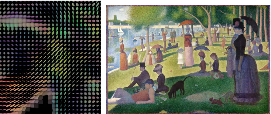
Figure 1.1: A diagram showing how DTI characterizes brain’s anatomical structure. The diagram is modified from Chung et al. (2011). Human brain has a complex anatomical structure (left). The structure can be non-invasive measured via characterizing the 3-D diffusion of water molecules (middle). The diffusion process is presented in terms of voxel-wise positive definite matrices visualized by ellipsoids (right).

neuroimaging techniques focusing on the brain’sfunction(e.g., functional MRI), DTI focuses on the brain’sstructure. DTI maps and characterizes the 3-D diffusion of water molecules as a function of the spatial location (Basser et al. 1994). The diffusion process in the brain reflects interactions with many obstacles, such as fibers, thereby revealing microscopic details about the underlying tissue architecture (Figure 1.1). The most intuitive understanding of DTI is that the voxel-level random variable is a 3×3 positive definite matrix (diffusion tensor or DT) describing the diffusion process (See Figure 1.2). This understanding motivates many statisticians to use positive definite matrix-variate models modeling DTs (Schwartzman 2006; Zhu et al. 2009; Yuan et al. 2012).

(15)

(a) A typical DTI: a 3×3 diffusion ten-sor in each voxel/pixel

(b) A Sunday Afternoon on the Island of La Grande Jatte: a univariate/RGB vector in each pixel

Figure 1.2: A comparison between DTI and ordinary images.

three spatial modelings oriented by three scientific objectives of DTI:

Covariate Effect Quantification: To understand covariate (age, gender, drug use,etc.) effects on the brain’s structure is a primary objective. An appealing method is the spatial Gaussian process model if the responses are real values. However, this model has not been extended to positive definite matrix-variate data. To mitigate it, we assume that the positive definite matrices follow Wishart distributions and use spatially continuous random fields supporting spatially dependent Wishart matrices. Based on theoretical results, we further simplified this model to a model composed of Gaussian processes. Both simulation results and real data analysis demonstrate the improvement utilizing the full matrix information, in comparison to univariate modeling. We introduce this geostatistical modeling in Chapter 2.

(16)

we further propose a Bayesian semiparametric mixture model of positive definite matrices, where the mixture labels follow a novel hierarchical Markov random field capturing spatial dependence. Finding regions of differences is simplified to testing if the discrete hierarchical variables are equal. Both simulation studies and real data analysis show a more accurate selection in comparison to univariate modeling. We introduce this Bayesian semiparametric model in Chapter 3.

Fiber Tracking: Another clinical objective is fiber tracking, depicting detailed anatomical connections of brain (Soares et al. 2013). Different from the previous two goals focusing on anal-ysis/inference, this objective can be considered to develop an imaging processing methodology. Following earlier works (Wong et al. 2016; Kang and Li 2016; Lazar et al. 2016; Schwartzman et al. 2016), we further simplify the parameterization quantifying uncertainties and use a spatial random field based on discrete spatial variation to incorporate spatial information. We use simulation studies and real data analysis to show an improvement in fiber direction estimation. This work is introduced in Chapter 4.

The three methods can be considered as an extension of classic spatial models (Gelfand et al. 2010a) including geostatistical modeling, spatial Bayesian nonparametric modeling, and spatial auto-regression to positive definite matrices. Therefore, these three methods not only resolve the clinical issues in DTI but also provide a comprehensive study ofspatial modeling of positive definite matrices.

(17)

CHAPTER

2 GEOSTATISTICAL MODELING OF

POSITIVE DEFINITE MATRICES

(18)

2.1 Introduction

Incorporating spatial dependence is important for achieving efficient and valid inference in imaging data analysis (Spence et al. 2007; Wu et al. 2013; Xue et al. 2018). Recently, Lan et al. (2019) also reveal that incorporating spatial dependence leads to improved performance in DTI region of difference selection, validated by an application to a cocaine user data (Ma et al. 2017). In point-referred data, geostatistical modeling is a useful approach. It is a class of models based on continuous spatial variation, providing a smooth surface over locations (e.g., spatial Gaussian process model). However, current geostatistical modeling only focuses on random variables following univariate or multivariate distributions (e.g., univariate/multivariate Gaussian, Poisson). However, the voxel-level variable in DTI is a positive definite matrix and only a few relevant works have been proposed for spatially-varying positive definite matrices (Gelfand et al. 2004). This triggers our study of geostatistical modeling of positive definite matrices.

(19)

(20)

spatially-varying coefficient process model (Gelfand et al. 2003).

To the best of our knowledge, this is the first work on exploring spatial associations in modeling positive definite matrix-variate data under the framework of geostatistical modeling, with some key theoretical contributions of multivariate analysis and applications to DTI. In the rest of the paper, we first introduce the spatial Wishart process model in Section 2.2; We next provide the Cholesky decomposition process model in Section 2.3; Sections 2.4 and 2.5 give simulation studies and real data application, respectively; Finally Section 2.6 concludes with a discussion. All the proofs and code are in supplementary materials.

2.2 Spatial Wishart Process Model

A typical DTI data set (e.g., Ma et al. 2017) usually includes DTs from each subject i∈ {1,2, ...,N}at each voxels∈ {s1, ...,sn}, and subject-level covariates (e.g., age and education years, medical treatments). The primary clinical objective is to detect local covariate effects on DTs. LetAi(s)be the 3×3 positive definite DT matrix of subjectimeasured at voxelsandXi be a design matrix containing an intercept anddcovariates. The positive definite DT matrices are modeled as parameterized Wishart matrices (Dryden et al. 2009) to have mean matrixΣi(s) and degrees of freedomm, denoted asAi(s)∼W(Σi(s),m). To model spatial dependence and ensure thatAi(s)is a positive definite matrix, we decomposeAi(s)as

Ai(s) =Li(s)Ui(s)Li(s)T. (2.1)

(21)

construc-tion forLi(s)as a function ofXiis described in Section 2.2.2. We refer this model as spatial Wishart process (SWP) model in the rest of the paper.

2.2.1 Residual Term: Spatial Wishart Process

In this subsection, we introduce the spatial Wishart process as a means of modeling spatial dependence. Gelfand et al. (2004) provide the construction of the spatial Wishart process, which is stated as follows. For j∈ {1,2, ...,m}, let{Zj(s):s∈D}be a mean-zero p-dimensional multivariate Gaussian process with p×pcross-covariance matrixΣand spatial dependence function K(s,s0|Φ) determined by parameters Φ(i.e., cov(Zj(s),Zj(s0)) =K(s,s0|Φ)×Σ), denoted asZ_jGP(0,K(s,s0|_Φ),Σ). If for eachs∈D, we collectU(s) =∑jZj(s)ZTj(s)/m, then the collection{U(s):s∈D}is a spatial Wishart process. The spatial Wishart process can be understood as a two-level hierarchical model where the spatial dependence of Wishart matrix

U(s)is induced by the latent spatial Gaussian processes{Zj}.

In applications, the number of locations in D is usually finite. However, Gelfand et al. (2010b) emphasize the importance to ensure a valid mathematical specification of a spatial stochastic process. Thus, in Theorem 1, we use the Kolmogorov extension theorem (Øksendal 2003) to prove that it is a valid stochastic process ifDis an uncountable collection of spatial locations (Appendix A).

Theorem 1. Spatial Wishart Process: The spatial Wishart process{U(s):s∈D}is a valid stochastic process (random field).

Based on the fact that the random field is valid, we can also show that this field is almost surely continuous (Proposition 1). The proof of almost surely continuity is based on Kent (1989) (Appendix A).

(22)

that goes to0at a rate of2+δfor someδ>0,U(s)converges weakly toU(s0)with probability

one as||s−s₀|| →0.

Considering that neuroimaging is usually is collected at a high resolution and the disease status at proximally-located/neighboring voxels can be similar (see Wu et al. 2013; Xue et al. 2018), the residualsUi(s)should be smooth and spatially dependent. Therefore, we model the residuals{Ui(s):s∈D}fori∈ {1,2, ...,N}as realizations of a spatial Wishart process with degrees of freedomm, cross-covariance matrixI, and correlation functionK(s,s0|Φ), denoted as

Ui∼SW P(m,K(s,s0|Φ),I). (2.2)

Setting the cross-covariance matrix toI preserves the designed marginal distributionA_i(s)∼ W(Σ_i(s),m).

In spatial statistics and neuroimaging, understanding the spatial dependence is essential. We quantify spatial dependence of the spatial Wishart process using the expected squared Frobenius normV(s,s0) =E||U(s)−U(s0)||2F, where||.||F is the Frobenius norm. The expected squared Frobenius norm can also be understood as a generalized variogram (Cressie 1992) for matrix-variate data (Lan et al. 2019), where an increasing spatial dependence ofU(s) and U(s0) leads to a smallerV(s,s0). Through the variogram, we find that the spatial Wishart process is separable (Cressie 1992) since

V(s,s0) =γ(m,Σ)[1−K(s,s0|Φ)2], (2.3)

(23)

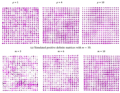
The result of spatial separability can be visually understood via realizations of the standard spatial Wishart processes (Σ=I) on a 20×20 grid with spacing of 1 between adjacent grid points. Given the spatial correlation function is exponentialK(s,s0|ρ) =exp

h

−||s−s0|| ρ

i , we visualize the positive definite matrices in two dimensions as ellipsoids in Figure 2.1. In Figure 3.3a, the positive definite matrices are simulated withm=3 andρ=1,4,10, where a largerρ leads to stronger spatial dependence; In Figure 3.3b, positive definite matrices are simulated withρ=4 andm=3,6,10, where a largermleads smaller cross-dependence. Since the three cases in Figure 3.3b maintain the same level of spatial dependence, we may also identify that the spatial and non-spatial variations are separable.

2.2.2 Regression Term: Cholesky Decomposition

Expressing the mean matrixΣi(s)in terms ofXiis not straightforward (Zhu et al. 2009; Yuan et al. 2012) because the responsesAi(s)are in a Remannian manifold but the covariatesXi are in Euclidean space. Following Zhu et al. (2009), we regress the(k,l)-th element ofLi(s), denoted asl_ikl(s)onXias

loglikk(s) =Xiβkk(s), likl(s) =Xiβkl(s) fork>l, (2.4)

where β_kl(s) = [β0kl(s),β1kl(s), ...,βdkl(s)]T is the spatially-varying coefficient vector and β_jkl(s) is the coefficient associated with the j-th covariate. The roles of the coefficients

βkl(s)can be explained as linear effect on loglikk(s) or likl(s). To model the spatial depen-dence of the mean effect, we assign a mean-zero spatial Gaussian process prior on β(s) = [β11(s)T,β22(s)T,β33(s)T,β21(s)T,β31(s)T,β32(s)T]T, denoted as

β∼GP(0,K(s,s0|_Φ_β),σ2

(24)

(a) Simulated positive definite matrices withm=10.

(b) Simulated positive definite matrices withρ=4.

Figure 2.1: Simulated positive definite matrices from standard spatial Wishart processes (i.e., with mean equal to the identity matrix). The spatial dependence of positive definite matrices depends on the range parameterρ. The cross-dependence of positive definite matrices depends on the degrees of freedomm.

2.3 Cholesky Decomposition Process Model

(25)

we further propose the Cholesky decomposition process (CDP) model. The CDP model is specified on the Cholesky decomposition elements ofA_i(s), denoted as{t_ikl(s):k≥l,s∈D}. The model is

Diagonal: √2 logt_ikk∼GP √

2X_iβ_kk(s),C(s,s0|_Φ_u),σ_m2

fork=1,2,3,

Off-Diagonal: t_ikl|¯t_ikk∼GP(Xiβkl(s),C(s,s0|Φu)t¯ikk(s)t¯ikk(s0),σm2) fork>l, (2.5) In the expression, √2X_iβ_kk(s) and X_iβ_kl(s) are marginal means of the diagonal and off-diagonal Gaussian processes at location s, respectively. Also, ¯t_ikk(s) =exp(Xiβˆkk(s)) and

ˆ

β_kk(s)is the ordinary least square estimates of a Gauss-Markov model (Monahan 2008, Section 4) for eachs:

logtikk(s) =Xiβkk(s) +εi(s); εi(s)∼N(0,σ2); i=1,2, ...,N.

To provide a rigorous mathematical validation, we also prove that{Ai(s) =Ti(s)Ti(s)T :s∈ D}is a valid stochastic process and almost surely continuous (Theorem 2), whereTi(s)is the lower-triangle Cholesky matrix.

Theorem 2. Cholesky Decomposition Process: {Ai(s) = Ti(s)Ti(s)T :s∈D} is a valid stochastic process. Also, if the correlation function C(s,s0|Φ)has a second-order Taylor series expansion with remainder that goes to0at a rate of2+δ for someδ >0,A(s)converges weakly toA(s0)with probability one as||s−s0|| →0.

(26)

mean oft_ikl(s);Φu controls the spatial residual dependence. Furthermore, if we modify that ¯

t_ikk(s) =exp(X_iβ_kk(s))in (2.5), the condition thatN→∞can be omitted. However, we show

that the specification in (2.5) leads to computationally efficient Gibbs sampling (Section 3.3) and a reasonable trade-off according to the simulation results showing the closeness of parameter estimation (Section 2.4).

Theorem 3. Asymptotic Properties: For i∈ {1,2, ...,N}, let{tikl(s):k≥l,s∈D}and{eikl(s): k≥l,s∈D}be Cholesky decomposition elements of{Ai(s):s∈D}following the CDP model and the SWP model, respectively. Fors1, ...,sn∈D, we have the following asymptotic results:

• Diagonal:As m→∞,

√

m[loge_ikk(s1)−Xiβkk(s1), ...,logeikk(sn)−Xiβkk(sn)]T d= √

m[logt_ikk(s1)−Xiβkk(s1), ...,logtikk(sn)−Xiβkk(sn)]T for k=1,2,3;

• Off-Diagonal:

– As m→∞, we have

E[[eikl(s1), ...,eikl(sn)]T|Seikl]

p −

→_E[[t_ikl(s1), ...,tikl(sn)]T|¯tikk] and

cor(e_ikl(s),e_ikl(s0)|Seikl)

p

−→K(s,s0|Φ)2=C(s,s0|Φ);

– Ifβ_kl(s) =0for alls∈D and k>l, then as m→∞and N →∞,

{√m[e_ikl(s1), ...,eikl(sn)]T|Seikl}

d

(27)

for k>l;

– Ifβ_kl(s) =0for alls∈D and k>l, andt¯_ikk(s) =exp(Xiβkk(s)), then as m→∞,

{√m[e_ikl(s₁), ...,e_ikl(s_n)]T|S_e_ikl}=d {√m[t_ikl(s₁), ...,t_ikl(s_n)]T|¯t_ikk}, for k>l;

d

= denotes for equal in distribution and −→p denotes for convergence in probability. Seikl(s)

is a partition of the latent Gaussian processes defined in spatial Wishart process{Zi j(s) = [Z_{i j}₁(s),Z_{i j}₂(s),Z_{i j}₃(s)]T :s∈D}for j∈ {1,2, ...,m}(i is a fixed and given index here). The partition is to take the dimensions “above" of e_ikl such as{[Z_{i j}₁(s), ...,Z_{i j}₍_k₋₁₎(s)]T :s∈D} for all j. For example,Sei31 or Sei32 is{[Zi j1(s),Zi j2(s)]

T _:_s_∈_D} _{for all j, and} _S

ei21(s) is {Zi j1(s):s∈D}for all j.

In comparison to the SWP model, the CDP model is a more feasible model with computa-tional convenience brought by Gaussian processes. Moreover, since the underlying mechanism of the DT’s spatial dependence is unknown, both models can be treated as proposed geostatistical models for DTI. On a higher perspective, given the asymptotic results, modeling Cholesky decomposition of Wishart matrices as Gaussian processes may be an efficient way to simplify many matrix-variate model for correlated Wishart matrices (e.g., Karagiannidis et al. 2003; Smith and Garth 2007; Kuo et al. 2007), bringing much computational convenience and avoiding complicated functions (e.g., hypergeometric functions, Bessel functions). All the proofs for the results in this section are summarized in Appendix B1-3.

2.3.1 Computational Details

(28)

correlation function, we defineρu,νu∈Φuas the range and smoothness parameter of the residual dependence, andρ_β,ν_β ∈Φ_β as the range and smoothness parameter of the mean dependence. We use priors logρu∼N(0,1), logρ_β ∼N(0,1), logνu∼N(−1,1)and logν_β ∼N(−1,1). We also assume thatσ−2

β ∼GA(0.01,0.01)andσ

−2

m ∼GA(0.01,0.01), which are conjugate priors allowing Gibbs sampling. The coefficientsβare also updated using Gibbs sampling because the posteriors are Gaussian distributions.

The computational bottleneck of the CDP model is factoring the large n×ncovariance matrix of the residual dependence and mean dependence, known as the O(n3) problem in spatial statistics. We address this problem using Vecchia’s method (Vecchia 1988), a local likelihood approximation that approximates the joint density of spatial variables as a product of conditional densities. Letω be an arbitrary Gaussian process. The approximated joint density is p[w(s1), ...,w(sn)] =∏sp[w(s)|w(s0),s0∈N(s)], whereN(s)is a set of neighboring locations of s(Datta et al. 2016). This reduces the computational complexity from O(n3)to O(nq3), where qnis the largest size ofN(s). This approximation is implemented fort_ikl, logt_ikk, andβ. A sensitivity analysis is presented in Section 2.4 to investigate the impact of the tuning parameterqon the CDP model.

2.4 Simulation

In this section, we first investigate the performance of the CDP model under data generated from either the SWP or CDP model, demonstrating that the CDP model produces reliable results under different geostatistical settings. Also, since we apply Vecchia’s approximation for fast computation, we conduct a sensitivity analysis to investigate the impact of q on parameter estimation.

(29)

Table 2.1: The spatial Gaussian process mean of the six coefficient vector for three covariates are summarized.Sis a set of spatial locations inside a 4×4 region in the middle of the image.

Covariate Diagonal Off-Diagonal

Intercept βint,kk=0, ∀s βint,kk=0, ∀s

x_i_,_drug βdrug,kk=0.5, fors∈S βdrug,kk =0, fors∈/S

βdrug,kl=0, ∀s

x_i,age βkk,age=0.25, ∀s βkl,age=0.25, ∀s

indicator x_i,drug∈ {0,1} and normalized age xi,age∈R+. The simulation study involves 50

replications. For each replication, there are 5 drug users (xi,drug=1) and 5 non-drug users

(xi,drug=0), andxi,ageis generated by a positive half-normal distribution (Leone et al. 1961)

with mean 0 and variance 1. For each replication, all the coefficients β are generated from a spatial Gaussian process with varianceσ_β =0.1 and correlation functionK(s,s0|Φ_β). The Gaussian process mean for three covariates (Table 2.1) simulates a scenario that drug has an effect on certain regions of the brain and increasing age may affect the whole brain. In all replications, we simulate the data withρu=ρ_β =2,νu=ν_β =0.5, andm=50. To investigate if Vecchia’s approximation with differentqaffects the model performance, we setq=10,50 and compare it to the model without Vecchia’s approximation. For each replication, we collect 5,000 MCMC samples after discarding 2,000 samples as burn-in.

The simulation results in terms of mean absolute deviation (MAD) of posterior mean estimates1, 95% posterior coverage2, and Monte Carlo standard deviation3 are summarized in Tables 3.1a and 3.1b. From the simulation result, we find that Vecchia’s approximation is acceptable since the computational times are 6 hours, 11 hours, and 35 hours for models with 10 neighbors, 50 neighbors, and without Vecchia’s approximation and MAD is nearly identical

1_|

E[θ|.]−θ|whereθis the true value andE[θ|.]is the posterior mean.

2_{Empirical percentage that the true value is in the 95% posterior}

3q1 T∑

T

(30)

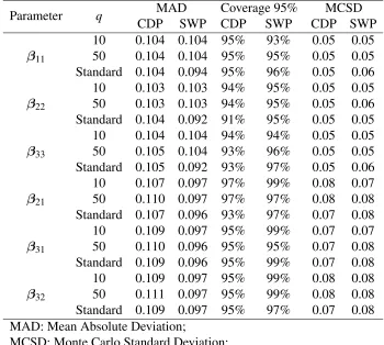
Table 2.2: Asymptotic (m=50) simulation results for spatially-varying coefficients with the data generated from the Cholesky decomposition process model or the spatial Wishart process model. The results are summarized in terms of mean absolute deviation of posterior mean estimates, 95% posterior coverage, and Monte Carlo standard deviation. The values are averaged over replications, voxels (n), and covariates (d).

Parameter q MAD Coverage 95% MCSD

CDP SWP CDP SWP CDP SWP

β11

10 0.104 0.104 95% 93% 0.05 0.05 50 0.104 0.104 95% 95% 0.05 0.05 Standard 0.104 0.094 95% 96% 0.05 0.06

β22

10 0.103 0.103 94% 95% 0.05 0.05 50 0.103 0.103 94% 95% 0.05 0.06 Standard 0.104 0.092 91% 95% 0.05 0.05

β33

10 0.104 0.104 94% 94% 0.05 0.05 50 0.105 0.104 93% 96% 0.05 0.05 Standard 0.105 0.092 93% 97% 0.05 0.06

β21

10 0.107 0.097 97% 99% 0.08 0.07 50 0.110 0.097 97% 97% 0.08 0.08 Standard 0.107 0.096 93% 97% 0.07 0.08

β31

10 0.109 0.097 95% 99% 0.07 0.07 50 0.110 0.096 95% 95% 0.07 0.08 Standard 0.109 0.096 95% 99% 0.07 0.08

β32

10 0.109 0.097 95% 99% 0.08 0.08 50 0.111 0.097 95% 99% 0.08 0.08 Standard 0.109 0.097 95% 97% 0.07 0.08 MAD: Mean Absolute Deviation;

MCSD: Monte Carlo Standard Deviation; SWP: Spatial Wishart Process Model;

CDP: Cholesky Decomposition Process Model.

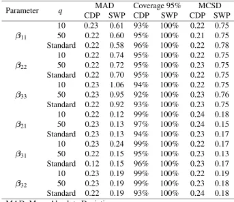
for all the three methods. We further conduct simulations withm=3 (Table 2.4 and 2.5). The closeness of parameter estimation is improved asmis larger validates the theoretical asymptotic results (Theorem 3)

(31)

Table 2.3: Asymptotic (m=50) simulation results for spatial parameters with the data gen-erated from the Cholesky decomposition process model or the spatial Wishart process model. The results are summarized in terms of mean absolute deviation of posterior mean estimates, 95% posterior coverage, and Monte Carlo standard deviation. The values are averaged over replications.

ρu=2

10 0.17 0.20 98% 98% 0.15 0.19

50 0.17 0.20 96% 96% 0.16 0.19

Standard 0.10 0.14 98% 96% 0.16 0.20 νu=0.5

10 0.033 0.033 98% 98% 0.035 0.027 50 0.033 0.033 98% 98% 0.032 0.029 Standard 0.022 0.022 97% 96% 0.040 0.031 ρ_β =2

10 0.13 0.13 98% 98% 0.20 0.25

50 0.13 0.13 98% 98% 0.20 0.24

Standard 0.10 0.13 98% 98% 0.21 0.25 ν_β =0.5

MCSD: Monte Carlo Standard Deviation; SWP: Spatial Wishart Process Model;

comprehensively but not concisely describe the local covariate effects, which may not be affirmative to clinicians who prefer scalar quantities (e.g., fractional anisotropy). However, since the six coefficients capture the covariate effects without information loss, our proposal is capable to accurately project the information onto any clinically meaningful scalar quantity. One of the useful quantities is fractional anisotropy, projecting a positive definite matrix onto[0,1], defined as

f_FA(A) = r

1 2

p

(λ1−λ2)2+ (λ2−λ3)2+ (λ3−λ1)2

q

λ₁2+λ₂2+λ₃2

, (2.6)

where{λ1,λ2,λ3}are the eigenvalues of a diffusion tensorA(Ennis and Kindlmann 2006). To

(32)

Table 2.4: Non-asymptotic (m=3) simulation results for spatially-varying coefficients with the data generated from the Cholesky decomposition process model or the spatial Wishart process model. The results are summarized in terms of mean absolute deviation of posterior mean estimates, 95% posterior coverage, and Monte Carlo standard deviation. The values are averaged over replications, voxels (n), and covariates (d).

β11

10 0.23 0.61 93% 100% 0.22 0.75

50 0.22 0.60 95% 100% 0.21 0.75

Standard 0.22 0.58 96% 100% 0.22 0.78

β22

10 0.22 0.74 95% 100% 0.22 0.75

50 0.22 0.72 95% 100% 0.23 0.75

Standard 0.22 0.70 95% 100% 0.22 0.75

β33

10 0.23 1.06 94% 100% 0.22 0.75

50 0.23 0.95 92% 100% 0.23 0.76

Standard 0.22 0.92 93% 100% 0.23 0.75

β21

10 0.22 0.12 99% 100% 0.24 0.18

50 0.23 0.13 97% 100% 0.24 0.15

Standard 0.23 0.13 94% 100% 0.23 0.17

β31

10 0.23 0.24 99% 100% 0.22 0.17

50 0.22 0.15 95% 100% 0.23 0.13

Standard 0.12 0.15 96% 100% 0.23 0.17

β32

10 0.23 0.19 99% 100% 0.22 0.19

50 0.23 0.19 99% 100% 0.23 0.18

Standard 0.22 0.19 93% 100% 0.24 0.18 MAD: Mean Absolute Deviation;

MCSD: Standard Deviation;

SWP: Spatial Wishart Process Model;

(33)

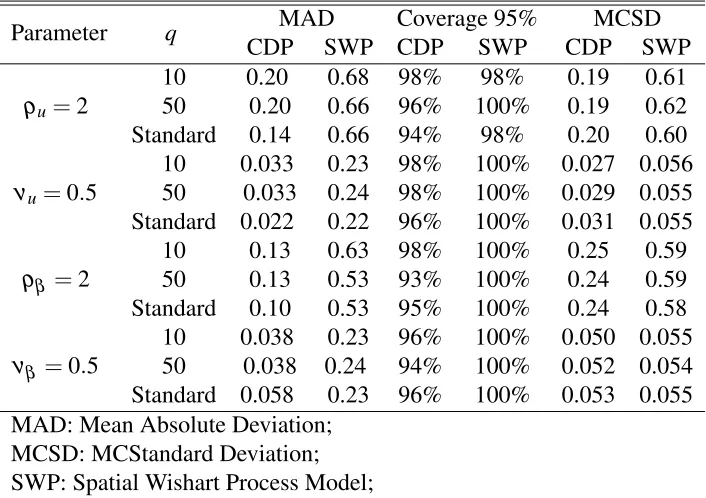
Table 2.5: Non-asymptotic (m=3) simulation results for spatial parameters with the data generated from the Cholesky decomposition process model or the spatial Wishart process model. The results are summarized in terms of mean absolute deviation of posterior mean estimates, 95% posterior coverage, and Monte Carlo standard deviation. The values are averaged over replications.

ρu=2

10 0.20 0.68 98% 98% 0.19 0.61

50 0.20 0.66 96% 100% 0.19 0.62

Standard 0.14 0.66 94% 98% 0.20 0.60 νu=0.5

10 0.033 0.23 98% 100% 0.027 0.056 50 0.033 0.24 98% 100% 0.029 0.055 Standard 0.022 0.22 96% 100% 0.031 0.055 ρ_β =2

10 0.13 0.63 98% 100% 0.25 0.59

50 0.13 0.53 93% 100% 0.24 0.59

Standard 0.10 0.53 95% 100% 0.24 0.58 ν_β =0.5

MCSD: MCStandard Deviation; SWP: Spatial Wishart Process Model;

as

ˆ

δFA(s) = 1 N

N

∑

i=1

E[fFA[Σi(s)]|xi,drug=1,rest]−E[fFA[Σi(s)]|xi,drug=0,rest]

, (2.7)

where the expectation can be empirically obtained by MCMC samples.

(34)

**** −0.2 −0.1 0.0 0.1 0.2

Univariate Model Working Model Model V alue Model Univariate Model Working Model CDP Model

(a)δFA(s)fors∈S.

−0.1 0.0 0.1 0.2

Univariate Model Working Model Model V alue Model Univariate Model Working Model CDP Model

(b)δFA(s)fors∈/S

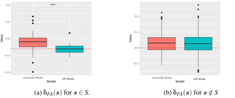
Figure 2.2: Estimates ofδFA(s)produces by the CDP model and the univariate model. The red dashed lines are the true values.

MCMC-based outcome regression estimator (Rotnitzky et al. 1998) is

ˆ

δFA(s) = 1 N

N

∑

i=1

E[f_logit−1 [yi(s)]|xi,drug=1,rest]−E[f_logit−1 [yi(s)]|xi,drug=0,rest]

, (2.8)

where yi(s)is response and flogit is the logit transformation. In Figure 2.2, the CDP model produces more precise estimates forδFA(s)fors∈Swith smaller uncertainties, revealing that utilizing the whole matrix information plays a key role in detecting covariate effects. This claim is further verified in real data analysis (see Figure 2.6).

2.5 Application to the Cocaine User Data

(35)

transferring motor, sensory, and cognitive information between the brain hemispheres. This region contains 15,273 voxels.

We first fit the data to the CDP model to investigate the covariate effects and spatial dependence among voxels. We set the design matrixXias

[1,xi,drug,xi,age,xi,edu,xi,handedness,xi,gender], representing the intercept, drug-use (xi,drug =1 if

subjectiis a cocaine user, otherwisex_i_,_drug=0), age, education years, handedness (xi,handedness=

1 if subjectiis a left-handed, otherwisex_i_,_handedness=0), and gender (xi,gender=1 if subjectiis

female, otherwisex_i_,_gender=0). We setq=50 for Vecchia’s approximation and totally 8,000 MCMC samples are collected after 3,000 samples as burn-in.

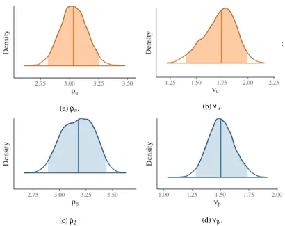
To understand the spatial dependence of the DTs, we plot the density histogram of the spatial dependence parameters ρu,νu, ρ_β, and ν_β in Figure 3.8, where the Bayesian mean estimates are 3.034, 1.75, 3.17, 1.51, respectively, and the 95% credible regions are[2.81,3.19], [1.39,1.93],[2.89,3.38],[1.28,1.67], respectively. The result reveals that the spatial dependence of the residual process and mean process are strong and smooth.

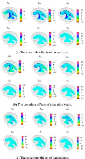
To compare the Bayesian mean estimates to 0 and quantify their uncertainties, the covariate effects on DTs expressed by their posterior z-scores4(Louis 1984) are visualized in Figure 2.4 and 2.5, which are smooth over voxels. Among these covariates, cocaine use is the covariate with the most significant impact, where the diagonal coefficients have many nonzero posterior z-scores located at some regions. The covariate effect of education years has no effect in most areas but a powerful impact at certain areas (seeβ11andβ31), which needs a further scientific

investigation. Unlike education years, the effect of age has a significant impact all over the corpus callosum, which may indicate the effect of age on brain structure is little but covers the whole area. Gender and handedness have comparatively small overall effects in comparison to the others but have strong effects in certain areas.

Furthermore, we use the MCMC-based outcome regression estimator to estimate the

drug-4E[θ|.]

(36)

(a)ρu. (b)νu.

(c)ρ_β. (d)νβ.

Figure 2.3: The posterior densities of spatial parameters for the cocaine user data.

(37)

(a) The covariate effects of age.

(b) The covariate effects of gender.

Figure 2.4: The covariate effects of biological attributes on DT expressing by the posterior z-scores of six spatially-varying coefficients.

reliability of our proposal.

2.6 Discussion

(38)

(a) The covariate effects of cocaine use.

(b) The covariate effects of education years.

(c) The covariate effects of handedness.

(39)

(a) The posterior z-scores ofδFAbased on the CDP

model.

(b) The posterior z-scores ofδFA based on the

uni-variate model.

Figure 2.6: The posterior z-scores ofδFA.

the Cholesky decomposition of positive definite matrices, overcoming the problematic issues caused by the intractable PDF of the SWP. Both the simulation studies and real data application demonstrate the novelty in spatial Bayesian inference of positive definite matrices.

(40)

which here is resolved by proposing the CDP model. Other attempts are mostly to investigate the special cases where the latent covariance matrix has a certain form (e.g., Mathai and Moschopoulos 1991; Furman 2008), compromising the flexibility. Meanwhile, Yu (2004) are proposing characteristic function-based parameter estimation approaches for models whose PDF is intractable but characteristic function is elegant. In Appendix A.1, we give the characteristic function of the spatial Wishart process which is simple and easy to handle, providing an alternative inference approach.

(41)

CHAPTER

3 BAYESIAN SEMIPARAMETRIC

MODELING OF POSITIVE DEFINITE

MATRICES

(42)

Statistics in Imaging.

3.1 Introduction

The spatial neuroimaging toolbox for univariate responses is considerably rich: Woolrich et al. (2004b) proposed a fully Bayesian model for spatiotemporal imaging data; Kang et al. (2011) implemented spatial point processes for meta-analysis of imaging data; To select essential biological features, Musgrove et al. (2016) introduced spatial Bayesian variable selection for neuroimaging data; Recently, Reich et al. (2018) proposed spectral methods for ADNI data to provide computational benefits. All of these studies demonstrated an improvement in the precision of estimates by properly accounting for spatial dependence.

In this vein, the Potts model, a generalization of the Ising model in statistical mechanics, has also been successfully applied to imaging (Johnson et al. 2013; Li et al. 2018). A desirable property of the Potts model is that it avoids smoothing over abrupt changes in the image intensity (Johnson et al. 2013), and this makes it more attractive than available Gaussian kernel methods. To this end, we assume the positive definite DTs follow a mixture of inverse Wishart distributions, with the mixture component labels modeled via a (spatial) Potts model, representing a discrete Markov random field. Thissemiparametric mixturespecification refers to a class of flexible mixture distributions with a finite number of components (Lindsay and Lesperance 1995).

(43)

two-wayframework, allowing hypothesis testing via group-level parameters and inter-subject variability simultaneously.

Our proposal is implemented using the Bayesian approach, accounting for the uncertainty of model parameters in all levels of the hierarchy. However, the Bayesian approach is often problematic in neuroimaging because of its heavy computational burden (Cohen et al. 2017). Although the associated Markov chain Monte Carlo (MCMC) algorithm is mostly composed of computationally tractable Gibbs steps that can be paralleled, a major drawback of the Potts model is the intractable normalizing constant, creating a bottleneck for hyperparameter updates. In this paper, it is resolved via the double Metropolis-Hastings algorithm (Liang 2010) recommended by Park and Haran (2018).

To the best of our knowledge, this is the first work on exploring spatial associations in modeling positive definite matrix-variate data under a Bayesian semiparametric framework, with applications to DTI. In the rest of the paper, we first introduce the single-subject and multi-subject model, and the group hypothesis testing framework in Section 3.2. Relevant MCMC computational details appear in Section 3.3. To demonstrate the improvement in performance compared to plausible alternatives, we perform simulation studies in Section 4.4. In Section 3.5, we present the application to the motivating cocaine data set. Finally, Section 3.6 concludes with a discussion.

3.2 Model

(44)

3.2.1 Single-Subject Model

LetAvbe thep×pDT at voxelv∈ {1,2, ..,n}. To ensureAvis symmetric and positive definite, it is usually parameterized as a (inverse) Wishart matrix (Dryden et al. 2009) or a Gaussian symmetric matrix-variate distribution (Schwartzman et al. 2008). In this paper, we assume that

Avfollows an inverse Wishart distribution as

Av|Mv,mIWp(Mv,m), (3.1)

whereIWp(Mv,m)is the inverse Wishart distribution parameterized (Appendix B.1) to have meanMvand degrees of freedomm>p+1, and the DTs are independently distributed acrossv given the mean matricesMvand the degrees of freedomm. The mean matrices are modeled as a finite mixture of Wishart distributions, denoted as[Mv|gv=k]:=Vkwheregv∈ {1,2, ...,K}is the latent cluster label. The prior ofVkisVkWp(Σ,ν)whereWp(Σ,ν)is the Wishart distribution parameterized (Appendix B.1) to have meanΣand degrees of freedomν >p.

Spatial dependence of the DTs is achieved through the dependence of the mean matrices

Mv. We induce spatial dependence via the latent cluster labels that follow a weighted Potts

model, specified via the full conditional distributions:

P_k=P(g_v=k|β,ηk,g−v)∝exp "

ηk+β

∑

u∈Nv

I(g_u=k) #

, (3.2)

whereg−vis the full setg={g1,g2, ...,gn}excludinggv,Nvis a set of indices of the neighboring voxels ofv, andI[A] =1 if eventAis true andI[A] =0 otherwise. Giveng−vbut marginal over g_v, the distribution ofAvis the mixture ofKinverse Wishart distributions:

K

∑

k=1

(45)

whereIW_p(A|V,m)is the inverse Wishart density function ofAwith the mean matrixV and the degrees of freedomm. Therefore, this semiparametric mixture model spans a rich class of density functions.

Via the Potts model, an image can be considered as a network whose nodes are the voxels. In this network, every voxel is connected to its neighboring voxels. The full conditional distribution ofg_vdepends only on the voxels in the neighboring setN_vand therefore the process is Markovian. Since the spatial parameterβ is the coefficient of the neighboring term∑u∈NvI(gu=k), the

spatial parameterβ controls the dependence on the neighboring voxels.

Unlike the classic Potts model (Wu 1982), the termsηkare added as offset terms controlling the overall mass on each cluster. We setηk=−kξ so the parameterξ >0 is the concentration parameter controlling the homogeneity of the latent cluster labels. It is problematic to pre-specify the number of componentsKin a mixture model (McCullagh et al. 2008) but the offset terms provide more weight on the key components and fewer weights on the trivial components. We fit the model by settingK to be an upper bound on the number of active clusters and allow the data to determine the number of active clusters via estimation ofξ: ifξ →0, there are several active clusters; ifξ is large, there are a few active clusters. As a result, the model is less sensitive to the number of componentsKwhen the offset termηkis included. This claim is verified in the simulation studies (Section 4.4) and the real data application (Section 3.5), where we find similar results for differentK.

Quantifying spatial dependence is a vital issue in spatial statistics and neuroimaging. Since this model is for matrix-variate data, we use the expected squared Frobenius norm to measure dependence. The dependence between matricesAandBcan be summarized asE||A−B||2F =

ETr[(A−B)T(A−B)]. The norm increases as dependence decreases. IfAandBare 1×1,

(46)

Figure 3.1: The density plot ofγ(m,ν,Σ)whenp=3 andΣ=I.

the expected squared Frobenius norm the variogram. For the Potts model described above, the variogram is

V(u,v) =_E||Au−Av||2F =γ(m,ν,Σ)P(u,v|β,ξ),

whereP(u,v|β,ξ)is the marginal (over all other cluster labelsg) probability ofg_u6=g_v, and γ(m,ν,Σ)is a measure of the variability inAv|Mvand variability ofVkacrossK. Therefore, the multivariate spatial dependence structure is separable (Cressie 1992) in that the dependence is the product of a non-spatial termγ(m,ν,Σ)that controls cross dependence and a spatial term P(u,v|β,ξ)that controls spatial dependence.

We give the expression ofγ(m,ν,Σ)in Appendix B.2. When p=3 andΣ=I, the non-spatial term has an expression that is 12(m+ν−4)(2m−7)

ν(m−3)(m−6) wherem>6 andν >3. Therefore, in

this special case, the cross dependence decreases ifmorν is larger (See Figure 3.1).

(47)

study the function. In Figure 3.2a, the function is computed under the scenario that the image is a 1-D grid withK =100 andξ =0. The spatial term P(u,v|β,ξ)increases with distance and larger spatial parameterβ leads to the stronger spatial dependence. We also compute the function value with differentKin Figure 3.2b. We have lim_|_u₋_v_|→_∞P(u,v|β,ξ) =1−_K1, where relevant result can be found in studies of extreme value analysis (see Reich and Shaby 2018). Increasing K leads to smaller spatial dependence. Hence, we fixK to be large to eliminate long-range dependence (e.g.,P(u,v|β,ξ)<1 for large|u−v|) and estimateβ to capture local dependence.

For a more intuitive understanding of this model, we also simulate the DTs and visualize the DTs as ellipsoids in a 40×40 grid. In these simulations, we useξ =0,m=4, andν =30. In Figure 3.3a, the DTs within the same latent cluster label are similar to each other, indicating that spatial dependence of the DTs can be achieved by the latent cluster labels following the Potts model. In Figure 3.3b, larger spatial parameterβ leads to a realization with more dependence on their neighbors. Figure 4.6 also illustrates that the Potts model allows sharp breaks, which is desirable if neighboring voxels are in different tracts.

3.2.2 Muti-Subject Model

Motivated by the cocaine users data set (Ma et al. 2017) that includes 11 cocaine users and 11 non-cocaine users, we extend the single-subject model to the multi-subject setting. The clinical objective is to analyze the brain’s physical structure for differences between the two groups. The objective can be statistically formulated as finding regions in the brain where the distribution of the DTs across the subjects is different between cocaine users and non-cocaine users.

(48)

0.00 0.25 0.50 0.75 1.00

1 2 3 4 5 6 7 8 9 10 11 12 13 14 15 16 17 18 19 Distance P(u,v| β , ξ ) β 10 2

(a)K=100

0.00 0.25 0.50 0.75 1.00

1 2 3 4 5 6 7 8 9 10 11 12 13 14 15 16 17 18 19 Distance P(u,v| β , ξ ) K 20 50 100

(b)β =10

Figure 3.2: Monte Carlo approximation of the spatial term P(u,v|β,ξ). The value varies depending on the distance|u−v|, the number of clustersK, and the spatial parameterβ;ξ =0.

DTs are conditionally independent given the random matricesMivfollowing a finite mixture model:

Aiv|Miv,mIWp(Miv,m), Miv:=Vgiv, VkWp(Σ,ν). (3.3)

(49)

(a) The left panel is the latent cluster labelsgv and each color denotes for a distinct

latent cluster label; The right panel is the corresponding simulated DTs.

(b) The panels from the left to the right are simulated DTs under the models with

β =1,2,6;K=20;ξ =0.

Figure 3.3: Simulated DTs based on the proposed model.

(50)

conditional distributions

P(giv=k|α,β,ξ,g−iv,h)∝exp

" −kξ₊

β

_∑

u∈Nv

I(giu=k) +αI(hxiv=k)

#

P(hxv=k|α,β,h−xv,g)∝exp

"

β

_∑

u∈Nv

I(hxu=k) +

∑

j:xj=x

αI(gjv=k) #

,

(3.4)

whereg₋₍_iv₎ is the set ongi={gi1, ...,gin}excludinggiv,h−(xv) is the sethx={hx1, ...,hxn} excludingh_xv,gis the set on{g1, ...,gN}, andhis the set on{h0,h1}. The joint probability mass

function (PMF) of{g1,g2, ...,gN} ∪ {h0,h1}is given in Appendix B.3. Since the conditional

densities in (3.4) satisfy the conditions of the Hammersley-Clifford Theorem (Clifford 1990), the existence of joint distribution of{g1,g2, ...,gN} ∪ {h0,h1}is guaranteed (Appendix B.3).

A graphical representation of this latent Potts model is provided in Figure 3.4. Cluster labelsgi andhx can be understood as the spatial pattern of subjecti and the general spatial pattern of subjects in group x, respectively. In comparison to the single-subject model, the group-clustering parameter α is introduced for modeling multiple subjects. Ifα =0,Aiv is independently distributed over subjects; otherwise, the subject-level cluster labelg_ivdepends on the group-level cluster labelh_x_i_v, leading to the smaller inter-subject variability of spatial dependence pattern within one group.

To further understand the role ofα andhxv, we inspect the density ofAivconditioned onhxv and marginal over all other labels (Appendix B.4). The conditional density ofAivgivenxi=x andhxv is the mixture of inverse Wishart distributions proportional to

K

∑

k=1

exp h

−kξ₊

αI(hxv=k) i

IW_p(Aiv|Vk,m), (3.5)

where the term exp h

−kξ₊

αI(hxv=k) i

(51)

Figure 3.4: The graphical representation of the latent cluster labels. The group-level cluster labels arehx={hx1, ...,hxn}and the subject-level cluster labels aregi={gi1, ...,gin}. Cluster labelshxandgiare mutually dependent. The subject-level cluster labelsgihave inter-subject variability. The group-level cluster labelshxare a summary of the spatial dependence of all subjects.

Assumingα>0, the conditional density (3.5) depends onxiif and only ifh0v6=h1v.

The clinical objective is to find regions of differences between two groups, which can be formulated into finding voxels for which the distribution ofAivis different forxi=0 orxi=1. As shown in the conditional density (3.5), the test can be simplified to the test that

Hov:h0v=h1v H_av:h₀_v6=h₁_v.

(3.6)

Bayesian inference provides estimates of the posterior probabilities of the hypotheses, which is further discussed in Section 3.3.

We investigate spatial dependence as in the single-subject model. To measure spatial depen-dence within and across subjects, we propose the variogram

(52)

(a) Individual variogram (b) Within-group variogram (c) Between-group variogram

Figure 3.5: Monte Carlo approximation of the spatial termPi j(u,v|α,β,ξ). The value varies depending on the distance|u−v|, the group-clustering parameterα, and the spatial parameter β;ξ =0.

inter-subject variogram, we also compare the within-group variogram for subjects withxi=xj and between-group variogram for subjects withxi6=xj. Both individual variogram and inter-subject variogram are also separable (Cressie 1992).γ(m,ν,Σ)is the non-spatial term which has been discussed in Section 3.2.1. The spatial termP_{i j}(u,v|α,β,ξ)is the marginal probability ofg_iu 6=g_jv.

(53)

3.3 Computation

We use MCMC to fit the model described in Section 3.2. The codes are written in hybridRand

C++codes. The final model is

Aiv|Miv,mIWp(Miv,m), Miv:=Vgiv, VkWp(Σ,ν)

P(g_iv=k|α,β,ξ,g₋₍_iv₎,h)∝exp

" −kξ₊

β

_∑

u∈Nv

I(g_iu=k) +αI(hxiv=k)

#

P(h_xv=k|α,β,h₋₍_xv₎,g)∝exp

"

β

_∑

u∈Nv

I(h_xu=k) +

_∑

j:xj=x

αI(gjv=k) #

(3.8)

which is referred to as the Potts Model in the rest of the paper. Using the moment method (Robert 2007)[Section 3.2.4], we set Σas the sample mean of all observed DTs. The priori information brought byΣ has a little impact if the number of observations is large. We put uniform prior for the degrees of freedommandν on[5,50]×[4,50]. Following Liang (2010), we put a uniform prior forθ={α,β,ξ}on[0,20]×[0,20]×[0,1], denoted asπ(θ). Below we describe the updating rule for each parameter.

The MCMC algorithm is a combination of Gibbs and Metropolis-Hastings steps. The latent mean matrices and cluster labels are updated via Gibbs steps. Their full conditional distributions are

• V_k|.∼W_p((Σ−1ν+ (m−p−1)∑i∑v:giv=kA

−1

iv )−1(Nnkm+ν),Nnkm+ν)

• P(giv=k|.)∝IWp(Aiv|Vgiv,m)exp

h −kξ₊

β∑u∈NvI(giu=k) +αI(hxi,v=k)

i

• P(hxv=k|.)∝exp

h

β∑u∈NvI(hxu=k) +α∑j:xj=xI(gjv=k)

i

(54)

To select regions of differences via Bayesian hypothesis testing, we reject the null hypothesis in (3.6) ifP(h₀_v6=h₁_v|.)<P(h₀_v=h₁_v|.). The posterior probabilities can be estimated through MCMC samples thath0v=h1vorh0v6=h1v.

Updating the Potts hyperparametersα,β, andξ is problematic because the normalizing constant in the joint distribution function of the cluster labels is intractable (see the joint PMF in Appendix B.3). A simple approach is to estimate the parameters outside of MCMC. The plug-in values can be obtained from cross-validation (e.g., Goldsmith et al. 2014), pseudo-likelihood comparison (e.g., Zhao et al. 2014; Lan et al. 2016), or by comparing empirical and model-based variograms (e.g., Figure 3.6 and 3.8). However, these methods fail to account for uncertainty about these imputed parameters and so we update them using the double Metropolis-Hastings algorithm (Liang 2010).

Park and Haran (2018) review several Monte Carlo methods for models with intractable normalizing constants and recommend the double Metropolis-Hastings algorithm proposed by Liang (2010) because of its ease of implementation and computational efficiency. Li et al. (2018) combine the double Metropolisâ ˘A ¸SHastings algorithm with usual Bayesian tools for implementing the Potts model. The double Metropolis-Hastings update for θ begins with a candidate θ0 drawn from q(θ|θe) where θeis the current value and q(θ|θe) is a log-normal random walk transitional probability centered atθe. Given the candidate θ0, we draw labels

g0_i={g0_iv, ...,g0_in}andh0_x ={h0_xv, ...,h0_xv}using Gibbs sampling for eachiandx, respectively. The candidate θ0 is accepted with the probability min(1,r) where r= π(θ0)P(g0,h0|θe)P(

e g,he|θ0)

π(θe)P( e

g,eh|θe)P(g0,h0|θ0)

(55)

3.4 Simulation

In this section, we illustrate the performance of our method using two simulation studies under different scenarios for synthetic data. We compare our method to the non-spatial DTI inference method the Gaussian symmetric matrix model (Schwartzman et al. 2008) referred to as the Ran-dom Ellipsoid Model. TheRandom Ellipsoid Modelis a non-spatial matrix-variate method and assumes thatA_ivfollows a Gaussian symmetric random matrix distribution with the probabil-ity densprobabil-ity function (PDF) as f(A_iv|x_i=x,Σ_v,σ2) =H(Aiv)exp

h

1

2σ2Tr(2ΣxvAiv−ΣxvΣxv) i

, whereΣxvis the DT’s population mean at voxelvof groupxandσ2is the nuisance parameter. TheRandom Ellipsoid Modelselects regions of differences via testingΣ0v=Σ1v, where the test statistics are constructed by maximum likelihood estimations. thePotts Modelhas 8,000 MCMC samples with 3,000 discarded as burn-in. Methods are evaluated in terms of true positive rate (TPR), false positive rate (FPR), false discovery rate (FDR), and typical computation time.

We first investigate the performance of our method when the data are generated from a mixture model. We use a 40×40 grid with spacing 1 between adjacent grid points as an image. Each simulated data set consists of 5 subjects in the control group (xi=0) and 5 subjects in the treatment group (xi=1). For the control group (xi=0), we equally partition the graph into 4 parts by rectangular regions so thatg_iv∈ {1,2,3,4}, ordered by right-to-left. Thus each region is a 40×10 region. The treatment group has the same partition as the control group, except a 10×10 region at the middle of the second region whereg_iv=5. This simulates the brain with a small region of difference between the two groups. For each simulation,Σk is generated based on the model

Σk∼W3((k+1)I3,30)fork=1,2,3,4; Σ5∼W3(1.5I3,30).

(56)

Our model withK=10,50,100 is compared to theRandom Ellipsoid Model. The results averaged over 50 data sets are summarized in Table 3.1a. Our model has significantly improved performance in terms of the TPR, FPR, FDR in comparison to theRandom Ellipsoid Model. The small number of subjects might be one of the causes that the alternative produces low TPR. Schwartzman et al. (2008) discusses that the accuracy of maximum likelihood estimates of the Random Ellipsoid Modelis dependent on the number of subjects. Since the choice ofK does not affect selection accuracy, the simulation results also support the claim that the model can be less sensitive to the number of clusters ifK is larger than the true clusters.

To determine robustness to model misspecification, we also simulate data from the spatial Cholesky process described as follows: The DT matrix for subjectiat voxelvis determined by six independent spatial Gaussian processesU_ivk(k∈ {1,2, ...,6}). These spatial Gaussian

processes are arranged in the lower triangular matrixL_ivwithL_iv=      

eUiv1 ₀ ₀ Uiv4 eUiv2 0

U_iv5 Uiv6 eUiv3

      . The

(57)

Table 3.1: The simulation results. The true positive rate, false positive rate, false discovery rate, and typical computation time of thePotts ModelandRandom Ellipsoid Modelare summarized.

(a) Data generated from mixture models

Method Potts Random

Ellipsoid K=10 K=50 K=100

TPR 0.99 0.97 0.98 0.29

FPR 0.013 0.010 0.009 0.00 FDR 0.025 0.025 0.024 0.002 Time (hours) 0.5 0.8 1.0 <0.01 (b) Data generated from the spatial Cholesky process

Method Potts Random

Ellipsoid K=10 K=50 K=100

TPR 0.79 0.80 0.77 0.50

FPR 0.01 0.01 0.01 0.00

FDR 0.03 0.03 0.02 0.03

Time (hours) 1.0 1.5 1.8 <0.01

A problematic issue to the use of Bayesian methods in neuroimaging data is their heavy computational burden. In both simulations, thePotts Modelhas a computational speed within a few hours. TheRandom Ellipsoid Modelavoids the expensive MCMC, but since the performance of theRandom Ellipsoid Modelis too conservative, thePotts Modelis a reasonable trade-off.

3.5 Real Data Application

(58)

(a) Individual variograms (b) Within-group variograms _{(c) Between-group variograms}

Figure 3.6: The empirical variograms of the cocaine users data (Ma et al. 2017). The lines are the empirical variograms for each subject/pair.

transferring motor, sensory, and cognitive information between the brain hemispheres (Ma et al. 2009). Conventionally, studies on cocaine use focus on this region (e.g., Ma et al. 2009, 2017; Lane et al. 2010).

Before model fitting, we examine the fit of the proposed model to the cocaine users data via empirical estimates of variograms. We denote ˆV_{i j}(d) = _N1

d∑|u−v|=d||Aiu−Ajv||

2

F as the empirical variogram value of subjectsiand j at distanced, whereN_d is the number of pairs with|u−v|=d. We plot these empirical variograms of the motivating data in Figure 3.6. The DTs have a strong within-subject spatial dependence (Figure 3.8a). The empirical within-group variogram (Figure 3.8b) also increases with distance, indicating inter-subject dependence within a group, however, the empirical variogram is almost flat in the between-group variogram (Figure 3.8c), which suggests that the subjects are independent if they are in different groups. Since these empirical variograms perfectly match the theoretical variograms in Figure 3.5, the the hierarchical Potts model assumptions about spatial dependence are reasonable.

(59)

Table 3.2: The Rand index for measuring clustering similarities. The off-diagonals of the table are the Rand indices for any twoK.

K 100 200 300 400 500

100 . 0.92 0.91 0.92 0.92

200 . . 0.94 0.95 0.94

300 . . . 0.96 0.95

400 . . . . 0.96

500 . . . . .

with K as 100, 200, 300, 400 and 500 and use the Rand index (Rand 1971) for measuring the similarities of regions of differences detection with differentK. The Rand index measures clustering similarity: if the two clusterings are almost identical, the index is close 1; otherwise, the index is close 0. In Table 3.2, the Rand indices of any two K are close to 1, hence the selection is not sensitive toK. For a concise illustration, we use the result ofK=100 in the rest of this section.

(60)

Figure 3.7: The regions of differences between cocaine users and non-cocaine users. This is the regions of differences selected by thePotts Model(left panel) and theRandom Ellipsoid Model(right panel). The red area is the regions of differences.

differences compared to alternative clinical studies on investigating the effect of cocaine use. For example, Ma et al. (2017) did not find such regions of differences by using the same data set.

The MCMC trace plots and posterior densities of the Potts spatial dependence parameters

(61)

(a) Group-clustering parameter,α

(b) Spatial parameter,β

(c) Concentration parameter,ξ

Figure 3.8: The MCMC summaries of the hyperparametersθ. The left panel is the histogram of posterior samples and the colored region is the 95% credible region. The right panel is the MCMC trace plot of posterior samples.

3.6 Discussion

(62)

model produces significantly improved performance compared to the non-spatial alternatives. The application to the DTI data set of cocaine users demonstrates the novelty of this model for detecting clinically meaningful regions of differences.

(63)

CHAPTER

4 FIBER TRACKING USING A SPATIAL

AUTO-REGRESSIVE MODEL

In this chapter, we introduce diffusion MRI fiber tracking using a spatial auto-regressive model. The corresponding paper is under working and it will be submitted toStatistical Methods in Medical Research.

Spatial Modeling of Positive Definite Matrices and Its Applications to Diffusion Tensor Imaging.

ABSTRACT

DEDICATION

BIOGRAPHY

ACKNOWLEDGEMENTS

TABLE OF CONTENTS

LIST OF TABLES

LIST OF FIGURES

CHAPTER

1

INTRODUCTION

CHAPTER

2

GEOSTATISTICAL MODELING OF

POSITIVE DEFINITE MATRICES

2.1

Introduction

2.2

Spatial Wishart Process Model

2.2.1

Residual Term: Spatial Wishart Process

2.2.2

Regression Term: Cholesky Decomposition

2.3

Cholesky Decomposition Process Model

2.3.1

Computational Details

2.4

Simulation

∑

∑

2.5

Application to the Cocaine User Data

2.6

Discussion

CHAPTER

3

BAYESIAN SEMIPARAMETRIC

MODELING OF POSITIVE DEFINITE

MATRICES

3.1

Introduction

3.2

Model

3.2.1

Single-Subject Model

∑

∑

3.2.2

Muti-Subject Model

∑

∑

∑

∑

3.3

Computation

∑

∑

∑

3.4

Simulation

3.5

Real Data Application

3.6

Discussion

CHAPTER

4

FIBER TRACKING USING A SPATIAL

AUTO-REGRESSIVE MODEL

4.1

Introduction

_∑

_∑

_∑

_∑

_∑