A RADIAL BASIS FUNCTION APPROACH TO
RETRIEVE SOIL MOISTURE AND CROP VARIABLES FROM X-BAND SCATTEROMETER OBSERVATIONS
R. Prasad
Department of Applied Physics Institute of Technology
Banaras Hindu University
Varanasi-221005, Uttar Pradesh, India
R. Kumar
Department of Electronics Engineering Institute of Technology
Banaras Hindu University
Varanasi-221005, Uttar Pradesh, India
D. Singh
Department of Electronics and Computer Engineering Indian Institute of Technology
Roorkee, (UA)-247667, India
Abstract—An outdoor crop-bed was prepared to observe scatterom-eter response in the angular range of 20◦ to 70◦ at VV- and HH-polarization. The soil moisture and crop variables like plant height, leaf area index and biomass of crop ladyfinger were measured at differ-ent growth stages of the crop ladyfinger. Temporal variation in scat-tering coefficient was found highly dependent on crop variables and observed to increase with the increase of leaf area index and biomass for both polarizations. In this paper, a novel approach is proposed for the retrieval of soil moisture and crop variables using ground truth mi-crowave scatterometer data and artificial neural network (ANN). Two different variants of radial basis function neural network (RBFNN) al-gorithms were used to approximate the function described by the input output relationship between the scattering coefficient and correspond-ing measured values of the soil moisture and crop variables. The new
model proposed in this paper gives near perfect approximation for all three target parameters namely soil moisture, biomass and leaf area index. The retrieval with minimal error obtained with the test data confirms the efficacy of the proposed model. The generalized regression network was observed to give minimal system error at a much lower spread constant.
1. INTRODUCTION
In the recent times, the applicability of microwave remote sensing has made significant headways for monitoring the soil and crop variables. A plethora of applications ranging from crop yield estimation, to the monitoring of crop variables have been tried successfully. The crop variables of interest generally include biomass, leaf area index, chlorophyll content, plant height etc. Soil moisture content being one of the most important parameters, its estimation becomes vital for improving yield forecasts, scheduling irrigation and other activities of crop management. The underlying principle behind the soil moisture estimation being the difference between the dielectric properties of wet and dry soil [1]. Leaf area index for a plant is a key functional determinant of energy, and exchange of CO2 becomes possible between
the attenuation parameters of various layers and inversion of this formulation is quite complex to retrieve the crop variables. Picard [9] has developed multiple scattering coherent models for understanding C-band radar backscatter from wheat canopy. In Picard [9] model, it is difficult to calculate multiple scattering interactions which increase the complexity of electromagnetic problem. Multiple scattering equations were applied to the case of vertical cylinders over an infinite surface. The major problem is to solve the multiple scattering equations.
Thus, these models are either very complex to solve or require a large number of input data to retrieve the crop variables and to understand the individual response of crop variables on microwave scattering/absorption. The quantitative understanding of the contribution by each crop variables to scattering, attenuation and the relative magnitude of the scattering from the soil and the vegetation is still a matter of debate for the most of crops.
Therefore, model free estimation techniques are the one which are capable of providing the best results be it a classification task or retrieval of crop-soil variables. The retrieval of crop variables using soft computational techniques becomes all the more important in the current technological scenario. Artificial neural networks (ANNs) hold a lot of promise in this field. Artificial neural networks are abstract computer systems which are inspired by biological nervous systems. Inspired by the enormous capability of the human brain to organize its structural constituents known as neurons, so as to perform certain computations many times faster than the fastest digital computers in existence today, neural networks try to mimic the aforementioned properties of the human brain by acting like a massively parallel distributed processor [10].
Radial basis function neural networks (RBFNN) have proved to be very good function approximators as well as classifiers for a wide variety of remotely sensed data. Generally the back-propagation algorithm [14] is widely recognized as a powerful tool for training of the multilayer neural networks (MLNN). But since it applies the method of steepest descent to update the weights, it often suffers for very slow convergence rates besides yielding suboptimal solutions [15]. In addition to the aforementioned limitation of MLNNs, the non-linearities associated with the network add considerable difficulties to theoretical analysis of the network behaviour [16]. RBFNNs provide us with a better alternative since they greatly reduce the training time. Since the number of radial basis neurons is equal to the number of training patterns, the practicability of RBFNNs gets confined to those problems which have limited number of patterns in low dimensional space [17].
In this paper, two variants of RBFNN algorithms namely conventional radial basis function neural network and generalized regression neural network (GRNN) were used for the retrieval of soil moisture content, biomass and leaf area index. The conventional RBFNN employed in the study utilized the newrb function in the MATLAB, whereas the newgrnn function is used to create the generalized regression network. The conventional radial basis network consists of two layers; one hidden radial basis layer of S1 neurons and
an output liner layer of S2 neurons. Radial basis network is created
iteratively by the newrb function. The neurons are added one by one to the network until the sum squared error falls beneath an error goal or a maximum number of neurons are reached. A generalized regression neural network (GRNN) is a specialized one for function approximation. The difference between the two lies in the architecture of the linear layer. In both variants, the spread constant is the most important parameter of the network. This determines the width of an area in the input space to which each neuron responds. When the spread is large enough, several radial basis neurons have fairly large output at any given moment. This makes the network function smoother and it results in better generalization.
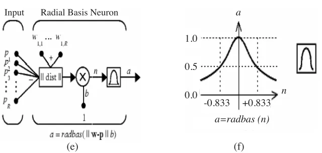
Figures 1(a) and 1(b) depict the structures of the two networks. As is evident from the Figs. 1(a) and 1(b), the difference between the weight vector of a neuron and its input vector should be minimized. This difference is denoted by the term ‘distance’. The radial basis neurons with their weight vectors quite different from the input vectors have near zero outputs. The vector IW1,1 represents the weight vector
generalized regression radial basis network, the LW2,1 is set equal to the target, and a dot product of the second layer weights with the output of radial basis layer is taken using the function nprod. One to one correspondence between the ‘distance’ and targets is more likely to be achieved using generalized regression radial basis networks and hence it becomes somewhat more suited to the function approximation problems than the conventional radial basis networks. The network
(a)
(b)
(e) (f)
Input Radial Basis Neuron
1.0
0.5
0.0
-0.833 +0.833
a=radbas (n) a
n
Figure 1. (a) A typical generalized regression radial basis function network with one radial basis layer and one linear layer. (b) A typical conventional radial basis function network. (c) Optimized ANN for training with one dimensional input vector for conventional RBFN and GRNN. (d) Optimized ANN for training with two dimensional input vector for conventional RBFN and GRNN. (e) A typical radial basis function neuron. (f) A typical radial basis transfer function curve.
The choice of spread constant being the most important parameter for the optimization of the network, the comparison between the two variants of the radial basis network, involves the study of generalization performance of the networks with different spread constants, for the retrieval of different target parameters.
2. MATERIALS AND METHOD
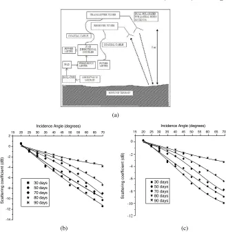
Ground based scatterometer measurements were performed to study the reflectivity/scattering coefficient of an outdoor crop-bed of crop ladyfinger at its various growth stages. Fig. 2(a) shows the schematic diagram of scatterometer system used in our field experiment. The height and incidence angle of the antenna mounted on the wooden platform can be varied. The height and look angle can be read from the graduated linear and circular scales with the pointers provided on the stand. The distance between the antennas and the centre of the target was selected in order to work in the far field region, and minimize the near field interactions. The polarization of radiated signal was changed by using 90◦ E-H twists. The scatterometer system was calibrated each day before and after microwave scattering measurement of crop ladyfinger. The measuring system was calibrated with help of an aluminium sheet of a known radar cross section. The radar cross section of the aluminium was calculated by using equation as
AlσP P(θ) =
4πA2
λ2
sin(kbsinθ)
kbsinθ
2
cos2θ, P =V orH, (1)
whereAlσP P(θ) is the radar cross section of the aluminium sheet,Ais
the area of the sheet,λis the wavelength of the incident wave,θis the incident angle,bis the dimension of the square sheet andk= 2λπ. The radar cross section of the aluminium sheet can be expressed in dB as
AlσP P(θ) = 10 log10[AlσP P(θ)], P =V orH. (2)
Firstly, the observations were carried out for aluminium sheet and the scattered power from the aluminium sheet was noted. After that scattered power was observed for crop ladyfinger at various growth stages in the angular range of 20◦ to 70◦ for both VV- and HH-polarizations. The scattering coefficient was calculated using equation
σP P0 (θ) = cropbedPP P
ALPP P ×Al
σP P(θ), P =V orH, (3)
(a) -14 -12 -10 -8 -6 -4 -2 0 2 Sca tte ring coe fficient (d B) 30 days 50 days 70 days 80 days 90 days
15 20 25 30 35 40 45 50 55 60 65 70
Incidence Angle (degrees)
(b)
15 20 25 30 35 40 45 50 55 60 65 70
0 -2 -4 -6 -8 -10 -12 Scattering coef ficient (dB) 30 days 50 days 70 days 80 days 90 days (c)
Incidence Angle (degrees)
Figure 2. (a) Schematic diagram of scatterometer system. (b)
Angular variation of scattering coefficient for crop ladyfinger at different stages of growth for VV-polarization. (c) Angular variation of scattering coefficient for crop ladyfinger at different stages of growth for HH-polarization.
In decibels, the scattering coefficient can be written as
σP P0 (θ)(dB) = 10 log1]
cropbedPP P
ALPP P ×Al
σP P(θ)
, P =V orH, (4)
leaf of crop ladyfinger was broad in shape and almost camouflaging the background surface on which it was grown. The fruit filling stage of this crop comes around 45±5 days from the date of sowing. The matured stage of this crop comes around 65±5 days. The age of the crop was counted from the date after sowing. Gravimetric soil moisture content of soil is determined by randomly choosing soil sample from the depth of 5 cm and taking the ratio of the weight of water present in the soil to the weight of the dry soil. LAI is defined as the ratio of total upper leaf surface of a crop divided by the surface area of the land on which the crop grows. LAI is dimensionless although it is some times presented in units of m2m−2. The biomass of the plant is the total dry matter accumulation in the complete plant over a period of time. The total biomass was computed from sample stalks and leaves, which were dried in oven at 90◦C for 24 hours. These samples were weight before and after drying and weight per square meter has been computed.
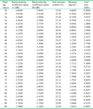
The obtained data was extrapolated using MATLABs polyfit function to provide us with sufficient data for approximation with the help of neural network as shown in Table 1. A set consisting of 30 data samples was obtained after extrapolating the data obtained from the scatterometer in the form of backscattering coefficient as inputs and soil moisture content, biomass content and leaf area index as targets parameters. The scattering coefficient was calculated both for sigma VV (vertical-vertical) and sigma HH (horizontal-horizontal) polarizations. Eighty percent of the data was used for training and twenty percent was used for testing purposes to assess the generalization capability of the proposed networks.
For the calculation of system error, the global statistical performance evaluation criterion “mean squared error” (MSE) was used for calculating the training phase and test phase error i.e.,
E(MSE) = Q1 Q
k=1
e(k)2, wheree(k) is the error andQis the number of
test set data. The performance of the trained network was evaluated by calculating the mean squared error calculated over the test data set for all three target parameters for both sigma VV and sigma HH polarizations. The networks with minimum training error were used in the testing of six test samples for each of the inputs. For both the variants of the RBFNN, the optimization of spread constant was done by varying its value from default “1.0” experimentally both in increasing and decreasing order and calculating the generalization error for each spread constant.
Table 1. All input and target parameters data.
Plant age (days)
Backscattering coefficient sigma vv (dB)
Backscattering coefficient sigma hh (dB)
Soil moisture content (%)
Biomass (Kg/m2)
Leaf area index
30 -4.6950 -3.9670 27.63 0.6650 0.9200
32 -4.6340 -3.9140 27.58 0.7042 0.9628
34 -4.5690 -3.8580 27.48 0.7478 1.0372
36 -4.5020 -3.7990 27.34 0.7958 1.1432
38 -4.4310 -3.7370 27.15 0.8482 1.2808
40 -4.3560 -3.6720 26.19 0.9050 1.4500
42 -4.2780 -3.6040 26.62 0.9662 1.6508
44 -4.1970 -3.5340 26.28 1.0318 1.8832
46 -4.1137 -3.4600 25.90 1.1018 2.1472
48 -4.0263 -3.3840 25.47 1.1762 2.4428
50 -3.9356 -3.3040 24.99 1.2550 2.7700
52 -3.8410 -3.2220 24.46 1.3382 3.1288
54 -3.7443 -3.1370 23.88 1.4258 3.5192
56 -3.6438 -3.0490 23.26 1.5178 3.9412
58 -3.5400 -2.9580 22.59 1.6142 4.3948
60 -3.4329 -2.8640 21.87 1.6900 4.8800
62 -3.3226 -2.7670 21.85 1.7112 5.1009
64 -3.2090 -2.6670 22.24 1.7328 5.2719
66 -3.0921 -2.5640 22.56 1.7488 5.4335
68 -2.9710 -2.4590 22.81 1.7652 5.5857
70 -2.8480 -2.3500 23.00 1.7800 5.7285
72 -2.7210 -2.2390 23.11 1.7932 5.8619
74 -2.5910 -2.1240 23.17 1.8048 5.9859
76 -2.4580 -2.0070 23.16 1.8148 6.1005
78 -2.3220 -1.8870 23.08 1.8232 6.2057
80 -2.1820 -1.7630 22.93 1.8300 6.3015
82 -2.0390 -1.6370 22.72 1.8352 6.3879
84 -1.8920 -1.5080 22.44 1.8388 6.4649
86 -1.7430 -1.3760 22.09 1.8408 6.5325
88 -1.5900 -1.2420 21.68 1.8412 6.5907
3. RESULTS AND DISCUSSION
The angular variation of scattering coefficient for crop ladyfinger at different growth stages are shown in Figs. 2(b) and 2(c) for VV- and HH-polarizations, respectively. The angular variation of scattering coefficient decreases (σ0) with the increase of incidence angle at each stage of crop ladyfinger for both the polarizations. However, angular variation ofσ0 was observed to decrease with the age of the crop. The angular variation of scattering coefficient between the incidence angles 20 to 70◦ is defined as dynamic range. The dynamic range of σ0 at different growth stage is quite different enough to discriminate the soil-moisture and ladyfinger effect. When the crop variables are small at the early stage, it is found that dynamic range ofσ0 is greater than in
the older age of crop. Soil moisture effect was observed to be dominant at early growth stage, when the magnitudes of the crop variables were less.
The dynamic range ofσ0 decreases with the age of crop shows the dominance of crop effect on soil moisture effect at 9.89 GHz. Thus, angular trends are more flat as the plant grows since the effects of soil is masked by developing vegetation. The dynamic range of σ0
at different growth stage is quite different enough to discriminate the soil-moisture and crop lady finger effect. The difference in crop covered soil moisture effect and crop effect at early and latter stage of crop is useful to analyze the data acquired by the space borne sensors. A comparison of angular variation of scattering coefficient was done with other research [18–21].
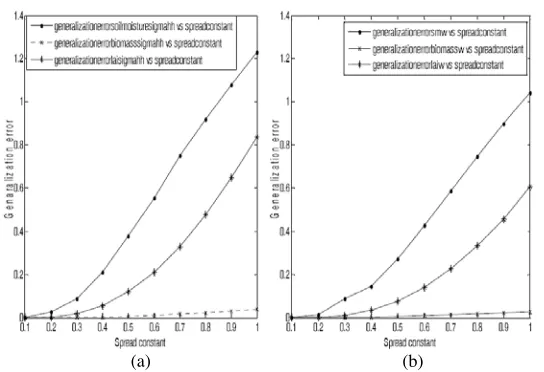
for all the three target parameters, in the sense that the error obtained at the optimized spread constant i.e., 2.0 was less when network was trained with VV-polarization data. In the case of generalized regression network, the optimized spread constant was 0.1 and almost zero error was obtained for all target parameter retrievals. The test performance of the network for the optimized spread constant of 0.1 was found to be similar for both VV- and HH-polarizations. The spread constant was varied from 0.1 to 1.0 in the increments of 0.1. Figs. 4(a) and 4(b) represent the variation in the generalization error with the change in spread constant for both GRNN and conventional RBFN. It can be concluded from these figures that the generalization error is lower for all three retrievals when the network was trained with GRNN. The variation in generalization error with change in spread constant is an important parameter to assess the efficacy of any network. The neural
(a) (b)
(e) (f)
(g) (h)
(k) (l)
Figure 3. (a) Observed and training output of soil moisture at
different growth stages (days) of crop for HH-pol. (b) Observed and training output of soil moisture at different growth stages (days) of crop for VV-pol. (c) Training output of GRNN for soil moisture retrieval for sigma vv-polarization. (d) Training output of GRNN soil moisture retrieval for sigma hh-polarization. (e) Biomass retrieval by conventional RBFN for VV-polarization. (f) Biomass retrieval by conventional RBFN for HH-polarization. (g) Biomass retrieval by GRNN for VV-polarization. (h) Biomass retrieval by GRNN for HH-polarization. (i) LAI retrieval by conventional RBFN for VV-polarization. (j) LAI retrieval by conventional RBFN for HH-polarization. (k) LAI retrieval by GRNN for VV-HH-polarization. (l) LAI retrieval by GRNN for VV-polarization.
Table 2. Observed values versus retrieved values with GRNN at
incident angle 45◦ for VV-polarization.
Plant age (days)
Backscattering Coefficient Sigma vv (dB)
Backscattering Coefficient Sigma hh (dB)
Soil Moisture (%) Target
Soil Moisture (%) Retrieved
Biomass Target (Kg/m2
)
Biomass retrieved (Kg/m2
) LAI target
LAI retrieved
38 - 4.4307 -3.7370 27.15 27.12 0.848 0.845 1.280 1.292
48 - 4.0263 -3.3840 25.47 25.47 1.176 1.160 2.442 2.440
58 - 3.5400 -2.9580 22.59 22.62 1.614 1.595 4.394 4.375
68 - 2.9720 -2.4590 22.81 22.76 1.765 1.763 5.585 5.573
78 - 2.3220 -1.8870 23.08 23.05 1.823 1.822 6.205 6.196
(a) (b)
Figure 4. (a) Variation in generalization error with spread constant for the target parameters using GRNN for HH-polarization. (b) Variation in generalization error with spread constant for the target parameters using GRNN for VV-polarization.
network selected for retrievals should always be less sensitive to the variation in learning parameters. The learning parameter in the case of a radial basis network is spread constant. Therefore a network which gives a constant error for a wide range of spread constants is considered better since designers can choose from a wide range of spread constant values for their network. Also, such network is more suitable for the VLSI on chip implementation. GRNN is found to have that property and therefore it is superior to the conventional RBFN.
4. CONCLUSION
This paper presents a method for the retrieval of crop-soil variables using scatterometer data incorporating RBFNN and GRNN as a computational tools. The retrieval values of biomass and leaf area index of crop ladyfinger were very much close to the observed values with almost zero system error at optimized spread constant without solving complex models and collecting numerous biophysical and soil parameters. In principle the study can be extended to different type of problems including classification of crop/vegetation. As the conclusion, we can summarize the following results:
both the conventional radial basis and GRNN algorithms.
• The generalized regression network gives minimal generalization error at a much lower spread constant than the conventional one. • The GRNN is less sensitive to the variation in spread constant
thereby giving the designers a wider choice.
• The error performance of the network using sigma vv polarization as the input is found to be better in both the variants of the radial basis network.
• The retrievals for biomass and leaf area index were found to be better than soil moisture content with almost zero system error at optimized spread constant.
REFERENCES
1. Jackson, T. J., J. Schmugge, and E. T. Engman, “Remote sensing applications to hydrology: Soil moisture,” Hydrological Sciences
Journal, Vol. 41, 517–530, 1996.
2. Bonan, G. B., “Importance of leaf area index and forest type when estimating photosynthesis in boreal forests,” Remote Sensing of
Environment, Vol. 43, 303–314, 1993.
3. Schmugge, T., “Remote sensing of soil moisture in hydrological forecasting,” 101–124, Wiley, Chichester, 1985.
4. Muukkonen, P. and J. Heiskanen, “Estimating biomass for boreal forest using ASTER satellite data combined with stand wise forest inventory data,” Remote Sensing of Environment, Vol. 99, 434– 447, 2005.
5. Schmugge, T. J., P. E. O’Neill, and J. R. Wang, “Passive microwave soil moisture research,” IEEE Transaction on
Geoscience and Remote Sensing, Vol. 24, 12–22, 1986.
6. Schmugge, T. and T. J. Jackson, “Mapping soil moisture with microwave radiometers,” Meteorology and Atmospheric Physics, Vol. 54, 213–223, 1994.
7. Wigneron, J. P., J. C. Calvet, T. Pellarin, A. A. Van de Griend, M. Berger, and P. Ferrazzoli, “Retrieving near-surface soil moisture from microwave radiometric observations: Current status and future plans,”Remote Sensing of Environment, Vol. 85, 489–506, 2003.
8. Cookmartin, G., P. Saich, S. Quegan, R. Cordey, P. Burgess-Allen, and A. Sowter, “Modeling microwave interactions with crops and comparison with ERS-2 SAR observations,” IEEE Transactions
9. Picard, G., T. L. Toan, and F. Mattia, “Understanding C-band radar backscatter from wheat canopy using multiple scattering coherent model,” IEEE Transactions on Geoscience and Remote
Sensing, Vol. 41, 1583–1591, 2003.
10. Hykin, S.,Neural Network a Comprehensive Foundation, 148–167, Prentice Hall, 1998.
11. Bishop, C. M., “Neural networks and their applications,” Review
of Scientific Instruments, Vol. 65, 1803–1832, June 1994.
12. Widrow, B. and M. A. Lehr, “Thirty years of adaptive neural networks: Perception, madaline and backpropagation,”
Proceedings of IEEE, Vol. 78, No. 9, 1415–1442, September 1990.
13. Loyola, D. G., “Application of neural network methods to the processing of earth observation satellite data,” Neural Networks, Vol. 19, 168–177, 2006.
14. Rumelhart, D. E. and J. L. McClellend, Parallel Distributed
Processing; Exploration in Microstructure of Cognition, MIT
Press, Cambridge, Mass., 1986.
15. Gori, M. and A. Tesi, “On the problem of local minima in backpropagation,” IEEE Transactions on Pattern Analysis and
Machine Intelligence, Vol. 14, 76–85, 1992.
16. Chen, F. C. and M. H. Lin, “On the learning and convergence of radial basis networks,” Proceedings of IEEE International
Conference on Neural Networks, 983–988, San Francisco, March
1993.
17. Daqi, G., W. Shuyan, and J. Yan, “An Electronic nose and modular radial basis function network classifiers for recognizing multiple fragrant materials,” Sensors and Actuators B, Vol. 97, 391–401, 2004.
18. Ulaby, F. T., R. K. Moore, and A. K. Fung, Microwave Remote
Sensing — Active and Passive, Vol. 2, 827–832, Addison Wesley,
Reading, MA, 1982.
19. Karam, M. A., A. K. Fung, and Y. M. M. Antar, “Electromagnetic wave scattering from vegetation samples,”IEEE Transactions on
Geoscience and Remote Sensing, Vol. 26, No. 6, 799–808, 1988.
20. Ulaby, F. T., T. E. Van Deventer, J. R. East, T. F. Haddock, and M. E. Colluzzi, “Millimeter wave bistatic scattering from ground and vegetation targets,” IEEE Transactions on Geoscience and
Remote Sensing, Vol. 26, No. 3, 229–243, 1988.
21. Singh, D., P. K. Mukhurjee, S. K. Sharma, and K. P. Singh, “Effect of soil moisture and crop cover in remote sensing,”