Accelerating ID-based Encryption based on Trapdoor DL
using Pre-computation
Hyung Tae Lee, Jung Hee Cheon, and Jin Hong
ISaC & Dept. of Mathematical Sciences, Seoul National University, 1 Gwanak-ro, Gwangak-gu, Seoul 151-747, Korea
{htsm1138,jhcheon,jinhong}@snu.ac.kr
Abstract. The existing identity-based encryption (IBE) schemes based on pairings require pair-ing computations in encryption or decryption algorithm and it is a burden to each entity which has restricted computing resources in mobile computing environments. An IBE scheme (MY-IBE) based on a trapdoor DL group for RSA setting is one of good alternatives for applying to mobile computing environments. However, it has a drawback for practical use, that the key gen-eration algorithm spends a long time for generating a user’s private key since the key gengen-eration center has to solve a discrete logarithm problem.
In this paper, we suggest a method to reduce the key generation time of the MY-IBE scheme, applying modified Pollard rho algorithm using significant pre-computation (mPAP). We also provide a rigorous analysis of themPAPfor more precise estimation of the key generation time and consider the parallelization and applying the tag tracing technique to reduce the wall-clock running time of the key generation algorithm.
Finally, we give a parameter setup method for an efficient key generation algorithm and estimate key generation time for practical parameters from our theoretical analysis and experimental results on small parameters. Our estimation shows that it takes about two minutes using pre-computation for about 50 days with 27 GB storage to generate one user’s private key using the parallelizedmPAPenhanced by the tag tracing technique with 100 processors.
Keywords:Identity-based Encryption, Trapdoor DL Groups, Discrete Logarithm, Pre-computation.
1 Introduction
In [26], Shamir suggested the concept of based cryptosystem and proposed identity-based signature schemes. Since then, there have been several proposals [9, 16, 28, 31] to con-struct an identity-based encryption (IBE) scheme. However, these proposals are not fully sat-isfactory. Some schemes require the condition that users cannot collude for the security and other schemes spend a long time to generate a user’s private key. Later, the first sufficiently secure and efficient IBE scheme was proposed using pairings by Boneh and Franklin [4]. Since Boneh and Franklin’s construction, many IBE schemes [3, 10, 33, 34] based on pairings have been proposed to enhance the security or efficiency. Also, some IBE schemes [2, 11] based on lattices have been also proposed under the necessary of lattice-based cryptosystems.
algorithm of lattice-based IBE schemes are more efficient than those of pairing-based IBE schemes, the public key size and private key size of lattice-based IBE schemes are quite large to utilize in mobile entities.
Among previous IBE schemes, Maurer and Yacobi’s suggestion is one of good alterna-tives for applying to mobile computing environments. In [16], the authors proposed a non-interactive key distribution (NIKD) algorithm based on a trapdoor DL group which is a maximal cyclic subgroup G of ZN∗ where an integer N is hard to factor. Also the authors
provided the IBE (MY-IBE) scheme from their NIKD algorithm. The most hard computation in encryption and decryption algorithms of the MY-IBE scheme is a modular exponentiation in ZN∗ and the user’s private key consists of one element less than N, hence, they are no
burden for a mobile entity.
However, the MY-IBE scheme has some problems for practical use. First, the security proof of the MY-IBE scheme is insufficient to formal security notion of IBE schemes, provided in [4]. Second, there are no secure full domain hash functions into a maximal cyclic subgroup GofZN∗. Moreover, the most serious obstacle for practical use of the MY-IBE scheme is that
the key generation time is quite long since the key generation center (KGC) has to solve a discrete logarithm problem (DLP) inGfor generating a private key of a user.
Later, Paterson and Srinivasan resolved the above three problems. In [20], they proposed a full domain hash function into G and proved the security of the proposed hash function. Then, they refined the MY-IBE scheme using their hash function and provided the security proof of the refined MY-IBE scheme based on the formal security definition of IBE schemes. Finally, they suggested that the use of the index calculus algorithm with significant pre-computation to reduce the key generation time. However, although KGC utilizes the index calculus algorithm with significant pre-computed data, there are no known concrete methods reducing DLP solving time and we cannot estimate the expected key generation time and required resources such as the amount of memory and the number of processors.
1.1 Our Contribution
The authors in [20] noted that there were no proper variants of the Pollard rho algorithm [23] using pre-computation. However there have been some proposals [12, 14] to reduce DLP solving time, modifying the parallelized Pollard rho algorithm [32] using pre-computation. In this paper, we suggest the method to reduce the key generation time of the MY-IBE scheme applying a modified Pollard rho algorithm using pre-computation (mPAP).
Also, we discuss about two extensions for reducing the wall-clock running time of the online phase in the mPAP. First, we consider the possibility of the parallelization of the
mPAPand provide the complexity analysis of the parallelizedmPAP. According to our anal-ysis, while the pre-computation phase of themPAPcan trivially be parallelized with speedup linear in the number of processors, the online phase of themPAPcan be parallelized with lin-ear increments of storage for speedup linlin-ear in the number of processors. Second, we consider applying the tag tracing technique [7] to themPAP for solving DLPs over a finite field. From experimental results, we confirm that the tag tracing technique works well with themPAP.
Lastly, we suggest a parameter setup method for reducing key generation time with main-taining security level and estimate the key generation time and the memory size of the MY-IBE scheme in the practical system from our theoretical analysis and implementation results on small parameters. According to our estimation on parameters for 280 security, the par-allelized mPAP enhanced by the tag tracing technique [7] requires about one minutes and 46 seconds with 100 processors when 100 processors are used for pre-computation for about 50 days with 27 GB storage. Since the key generation process is performed by the key gen-eration center, 100 processors are quite practical.
1.2 Organization
We introduce the MY-IBE scheme and give some related works on DL algorithm using pre-computation in Section 2. Section 3 describes the mPAP and provides more rigorous com-plexity analysis of the algorithm. We also give experimental results on small parameters and consider the parallelization and applying the tag tracing technique. In Section 4, we suggest a parameter setup method for reducing key generation time and estimate the key generation time of the MY-IBE scheme from our theoretical analysis and experimental results on small parameters.
2 Preliminaries
In this section, we introduce an identity-based encryption scheme (MY-IBE) based on trap-door DL groups for RSA setting, proposed by Maurer and Yacobi [16] and refined by Paterson and Srinivasan [20].
The key generation center has to solve one DLP in the key generation algorithm of the MY-IBE scheme and it takes a long time for practical use. To reduce the key generation time the authors of [20] suggested the re-use of significant pre-computed elements for solving previous DLPs. However, their suggestion was not enough to make the MY-IBE scheme practical for real systems. At the end, we briefly introduce related works on our suggestion to solve DLPs using significant pre-computation, which is a modification of the parallelized Pollard rho algorithm [32].
2.1 Identity-based Encryption based on Trapdoor DL
Definition 1 ( [8] ). We define the two following algorithms:
– TDLGen : a polynomial-time algorithm which takes as input a security parameter λ and outputs a finite cyclic group G, a generatorg of G and its trapdoor information τ. – SolveTDL : a polynomial-time algorithm which takes as input a finite cyclic group G, a
generatorg of G, a trapdoor information τ and a target element h of a DLP and outputs the DL of h based on g.
We also define a polynomial-time algorithmGenwhich takes as input a security parameterλ, runsTDLGen(λ) algorithm and then outputs(G, g). If (G, g, τ) is an output of TDLGen and a DLP over Gis hard for the output of Gen, we call G a trapdoor DL group.
As examples of trapdoor DL groups, one considers a maximal cyclic subgroup G of Z∗N whereN is a product of primes and its trapdoor information is the factorization of N [16]. Then one who knows a factorization of N can efficiently solve a DLP over G using Index Calculus algorithm or Pohllig-Hellman algorithm with Pollard rho algorithm. However, ifN is a product of more than three primes, there are no secure full domain hash function intoG. Also, one may consider trapdoor DL groups over an elliptic curveE(F2161), whose trapdoor information are isogenies [30]. But an elliptic curve E(F2161) is the only currently known possible parameter and it is not yet known how to generalize construction to higher security level.
In this paper, among these trapdoor DL groups, we will only deal with a maximal cyclic subgroupG of Z∗N where N is a product of two primes p, q that are roughly the same size and satisfy p≡3 (mod 4),q≡1 (mod 4), andp−1, q−1 are B-smooth integers.
Note thatTDLGen and SolveTDLare both polynomial-time algorithms in the above def-inition. To our knowledge, there are no polynomial-time algorithms to solve a DLP in a maximal cyclic subgroup G of ZN∗ although the trapdoor information is given. Hence, the
above group G does not satisfy the definition of trapdoor DL groups. However, there are some algorithms to solve DLP over G, whose complexity is sub-exponential or exponential in the security parameter λ but it is quite practical. Hence, we will apply the definition of
SolveTDLrelaxedly.
Identity-based Encryption based on trapdoor DL groups In [16], Maurer and Yacobi proposed an IBE scheme based on a trapdoor DL groupGwhich is a maximal cyclic subgroup ofZN∗ where N is a product of primes and whose trapdoor information is a factorization of
N. However, whenN is a product of more than three primes, the authors could not give an efficient full domain hash function from a set{0,1}∗ toG. Also, although they presented two
efficient full domain hash functions from{0,1}∗ toG whenN is a product of two primes, it was proved that their suggestions were not secure [15, 17–19]. In [19], the authors presented another full domain hash function into G, however they did not give a security proof of the presented hash function.
se-cure IBE scheme based on the security notion in [4]1. Here, we present the MY-IBE scheme modified by Paterson and Srinivasan. The scheme consists of four algorithms:
– Setup(λ): this algorithm runsTDLGenalgorithm to obtain (G, g, τ) whereGis a maximal cyclic subgroup of ZN∗, g is a generator of G and trapdoor information τ which is a
factorization of N. (We assume thatN is a product of two primes that are roughly the same size and satisfyp≡3 (mod 4),q≡1 (mod 4) and gcd(p−1, q−1) = 2.) LetH be a hash function from {0,1}∗ toZ
N and defineH1 :{0,1}∗→G by
H1(ID) =
H(ID) N
H(ID)
where Nx
denotes the Jacobi symbol. Let H2 :G→ {0,1}` be a hash function where ` is the bit size of messages. Then this algorithm outputs
params= (λ, G, N, g, H, H1, H2, `)
msk=τ = (p, q).
– KeyGen(params,msk,ID): this algorithm computesH1(ID). Then it runsSolveTDL(G, g, τ, H1(ID)) and obtains the private keysID such thatgsID=H1(ID). It outputssID.
– Encrypt(params,ID, M): this algorithm computes H1(ID) and chooses r ∈ ZN uniformly
at random. Then it outputs C= (U, V) where U =gr and V =M⊕H2(H1(ID)r). – Decrypt(params,sID, C): for a ciphertext C = (U, V), this algorithm outputs M0 = V ⊕
H2(UsID).
Note that the above scheme is IND-ID-CPAsecure under the CDH assumption and one-wayness of the hash function H1. Also the CDH problem in the above group G is at least hard to factorN. Therefore, the above scheme isIND-ID-CPAsecure if factoring N is hard.
Although the encryption and decryption algorithms are efficient since those require two and one modular exponentiation, respectively, KGC has to solve one DLP overGto generate the private key for one user. Hence, the weak point of the above scheme is to spend a long time in the key generation algorithm. To overcome this obstacle, the authors in [20] suggested the use of the index calculus algorithm with a large amount of pre-computation.
2.2 Discrete Logarithm Algorithm using Pre-computation
To reduce key generation time in KeyGen algorithm of the MY-IBE scheme, the authors in [20] suggested the use of the index calculus algorithm [1] with significant pre-computation over Zp and Zq for solving a DLP in a maximal cyclic subgroup G of ZN∗ where N = pq
and p, q are primes. The index calculus algorithm for solving DLPs divides into two parts, the pre-computation phase and the online phase. In the pre-computation phase, when the cyclic group G and a generatorg are given, one computes DLs of all elements in the factor baseB. Then in the online phase, one finds some relations between the target element of the
1
DLP and elements in the factor base B and then solves the DLP using DLs of elements in the factor baseB, which are pre-computed in the pre-computation phase.
However, the complexity of the online phase is the same with the complexity of the pre-computation phase in the original index calculus algorithm. Hence, it also requires a large amount of computations for the online phase. For achieving 80-bit security, we assume that the bit size of p and q is 512. Then, according to the analysis of the number field sieve method [6] which is a variant of the index calculus algorithm, it is required about O(278.04) multiplications2 inZp andZq in the online phase and hence it is impractical to realize in the
system.
To make the MY-IBE scheme more practical, we will propose the use of the Pohlig-Hellman algorithm and the modified Pollard rho algorithm with a large amount of pre-computation. In [20], the authors noted that there were no proper algorithms to solve DLPs using the Pollard rho algorithm with pre-computation. However, there have been some mod-ified Pollard rho algorithms [12, 14] to solve a DLP efficiently using pre-computation. In [14], the authors provided the algorithm for solving multiple DLPs using elements which were computed for solving previous DLPs, modifying the parallelized Pollard rho algorithm [32]. Then the authors in [12] modified the above multiple DLPs solving algorithm to the DLP solving algorithm with pre-computation, by solving randomly generated DLPs before the target element of the original DLP is given.
In the rest of this section, we introduce some basic concepts,r-adding walk iterating func-tion and distinguished point (DP) collision detecfunc-tion method, which are composing variants of Pollard rho algorithm.
WhenGis a cyclic group of orderqgenerated by a generatorg, if we know the factorization ofq=Q`
i=1p
ei
i wherepi’s are primes, one can reduce the DLP over Gto DLPs over a group
of orderpi’s using the Pohlig-Hellman algorithm. Hence, it is assumed that the group order
q is prime from here in this subsection. The group elementh denotes the target element of the DLP, in other words, we are looking for the value loggh.
r-adding walk iteration function We briefly look into r-adding walk iterating functions. Par-titionGinto r roughly same sized subsetsG1,· · ·, Gr so thatG=G1∪ · · · ∪Gr. The index
functions:G→ {1,2,· · · , r}is defined to be almost pre-image uniform and efficiently com-putable. Then chooser pairs (ui, vi) ∈Zq×Zq and set r multipliers Mi toguihvi. (In [12],
the authors suggested the use of multipliers which are independent of the target element. Hence we will set multipliers of r-adding walk iterating function in the mPAP to the form guih0 whereu
i is a randomly chosen integers in Zq.) Define r-adding walk iterating function
Fr :G×Zq×Zq →G×Zq×Zq by
Fr(y, a, b) = (y·Ms(y), a+us(y), b+vs(y))
wherey=gahb. Throughout this paper,Fr will denote anr-adding walk iterating function.
2
The heuristic complexity of the number field sieve for solving one DLP over Zp∗ is exp((c +
It was shown [25] that the expected number of iterations for finding a collision in a walk generated byr-adding walk for r ≥8 is O(√q). Experimental results [29] over elliptic curve groups show that the expected number of iterations required to find a collision with 20-adding walk is very close to
q
q
2π, which is that with a random function.
DP collision detection method Let us introduce the DP technique [24], which was originally used in time memory tradeoff techniques. One sets the distinguishing property that is easy to check and define a DP by a point satisfying the distinguishing property inG. For example, one may define the distinguishing property to be that a certain number of the most significant are all zeros under a fixed encoding ofG. One starts with an empty table, and the walk is computed iteratively until the walk encounters a DP. Then one searches for the same point with the occurred DP in the table. If it is not in the table, one stores it and generates another walk. The DP collision detection method is required abouttadditional iterations for noticing a collision after a collision occurs in a walk whent−1 is the proportion of DPs inG. It is straightforward to apply the DP method to multiple walks, so the DP method has an advantage that admitsn-times speedup with ann-processor parallelization [32].
3 Analysis of Discrete Logarithm Algorithm using Pre-computation
In this section, we describe the mPAP, which is a modification of the parallelized Pollard rho algorithm [32]. Then, we provide more rigorous complexity analysis of the algorithm and give experimental results on small parameters. Finally, we consider two extensions to reduce wall-clock running time of the online phase in themPAP, the parallelization of themPAPand applying the tag tracing technique.
3.1 Algorithm Description
Now, we are ready to describe themPAP, which is a modification of the parallelized Pollard rho algorithm [32]. Our description is modified in three points compared with the algorithm in [12]. First, in the pre-computation phase one generates chains which are started from a random starting point and are ended at a DP, not randomly generating DL instances and solving these DLPs. Second, multipliers of anr-adding walk iterating function are given by a special form. Third, one does not store created DPs in the online phase because its advantage is almost negligible.
Let us describe the mPAP. Choose positive integers m, tsuch that mt2 =αq wherem is the number of generated chains in the pre-computation phase,t−1 is the proportion of DPs in the group, andα is not a large constant. The parameters are assumed not to be extreme, in the sense that 1m, tqand a typical value isα≈1. We shall later determine the proper size of parametersm, t, α. Fix an r-adding walk iterating functionFr so that the multipliers
have the formguh0for some randomu∈Zq. Since the pre-computation phase starts before a
target element is given, the multipliers of ther-adding walk iterating functionFr must have
In the pre-computation phase, one choosesm random starting pointsgi,0 =gai,0h0 ∈ G for 1≤i≤mand iteratively computesgi,j+1=Fr(gi,j). Each chain is terminated at its first
encounter with a DP. We call by a DP chain a chain ended at a DP. Then one stores the occurred DPs and the exponents corresponding to each DP in a DP tableDT.
The average number of iterations to generate a DP chain ist, but some of chains may fall into a loop that never reaches a DP. In order to detect a chain falling into an infinite loop, we set a chain length bound ˆt. Any chain longer than this bound is discarded and one can choose to regenerate a chain from a different starting point. Note that the probability for a chain not to reach a DP until its ˆt-th iteration is (1− 1
t)
ˆ
t+1 ≈exp(−tˆ+1
t ). This shows that
setting ˆtto a reasonable multiple oftwill suffice in removing the effect of any such discarded chains for any practical purpose.
After the pre-computation phase, one obtains the following matrix.
g1,0
Fr −→g1,1
Fr
−→ · · · Fr −→g1,t1
g2,0
Fr −→g2,1
Fr
−→ · · ·−→Fr
g2,t2 ..
. gm,0
Fr −→gm,1
Fr
−→ · · · Fr −→gm,tm
Such matrix consisting ofmDP chains is called the DP matrix.
In the online phase, when a target element h of DLP is given, one starts to generate a DP chain from an element hr for a random 1≤ r < q. When a DP occurs in a chain, one compares it with the stored DPs in the table DT. If a collision is not found, one generates another DP chain from a distinct starting pointhr0 for a random 1≤r0 6=r < q. Otherwise, one can get the DL ofh from the relation ai ≡xbj +aj (modq) where x is the DL of h, a
pair (gi, ai, bi) and (gj, aj, bj) is the collision, (gi, ai, bi) is the stored point in the table DT,
and (gj, aj, bj) is the created DP in the online phase.
In the modification of the mPAP described in [12], created DPs in the online phase are also added to the DP tableDT. However, unlessαis not extremely small, the number of newly created DPs in the online phase is just one or two. It does not give a big help of accelerating DL computation of a present target element and hence we do not consider saving created DPs in the online phase.
3.2 Complexity Analysis
The analysis of themPAPcan be inferred from DL algorithm [14] for multiple instances. Ac-cording to the analysis, the expected number of group operations to solvekDLPs sequentially with their algorithm is about √2kq. From these results, we simply guess that the expected number of group operations to solve the (k+ 1)-th DLP is about √2q/(√k+ 1 +√k) =
p
Moreover, Hitchcock et al. [12] provided the expected online time complexity of the
mPAPassociated with the amount of pre-computation. However, their analysis has two miss-ing points:
– Although collisions may occur in the pre-computation phase, it does not consider this fact in their analysis. Hence they regard that the number of distinct elements in a DP matrix is the same with the number of iterations in the pre-computation phase.
– It does not consider the additional iterations to reach a DP for collision detection after a collision occurs in the online phase.
Now, let us correct the complexity of the mPAP. We shall exploit the analysis technique of time-memory tradeoff. Recently, in [13], the authors gave the expected number of distinct entries in a DP matrix for various ˆt. However, it does not give an error bound of the ap-proximation value. In the following lemma, we present the precise limit value of the expected number of distinct entries in a DP matrix when ˆtis sufficiently large and provide the differ-ence between the limit value and the expected number when we use a specific ˆt. This lemma will make up for the first missing point of the analysis provided by Hitchcock et al.
Lemma 1. Consider a DP matrix created with parameters satisfying mt2 =α q. When the iterating function is taken to be the random function andtˆis sufficiently large, we can expect the DP matrix to contain
q
1 + 2α+O(1t)−1
α m(t−1). (1)
distinct entries. Moreover, the difference between the expected number of distinct entries con-tained in the DP matrix and the above limit value is bounded bym(ˆt+t) exp(−ˆt/t).
Proof. We follow the proof of Proposition 10 provided in [13]. Consider a DP matrix generated in the pre-computation phase. Letmj be the number of elements which first appear atj-th
column in a DP matrix. Now we assume that chains not reaching a DP until ˆtsteps remain on a DP matrix for an analysis and however we will give the error bound considering that these chains are discarded. Then the recurrence relation
mj
q =
1−exp
−
mj−1
q 1−
1 t
1−
Pj−1
i=0mj q(1−1/t)
!
with m0 = m is satisfied from Lemma 6 in [13]. Differently from the analysis of [13], the initial value of the sequence (mi)∞i=0 is m since our DP table are generated from the exact
mstarting points without making up for the discarded chains to store the exactm DPs in a table.
Letµi =
mi
q(1−1/t) and σj =
Pj−1
i=0 µi. Then the recurrence relation
σj+1−σj =
m0
q −
1 tσj−
1 2σ
2
j +O
1 t3
is also satisfied from Lemma 7 in [13]. The sequence (σj)∞j=0 is monotone increasing from
the definition of the sequence (σj)∞j=0 and all σj’s are bounded since the sum P∞i=0mj does
not exceed the group orderq. Hence the sequence (σj)∞j=0 converges and the limit S of this
sequence is −1 t + s 1 t 2 + 2 m q +O
1 t3
and allσj’s are less than S. Therefore, the expected number of distinct entries in a DP table
is
∞ X
i=1
mi=q(1−1/t)
−1 t+ s 1 t 2 + 2 m q +O
1 t3 (2) = q
1 + 2α+O(1
t)−1
α m(t−1). (3)
LetE be the expected number of distinct elements in a DP table that chains whose length exceeds ˆt are discarded. Then,
E≤
ˆ
t
X
i=1
mj ≤q(1−1/t) lim j→∞σj
=q(1−1/t)S≤ √
1 + 2α−1
α m(t−1).
Now, we consider the lower bound of E. Note that the probability that a chain reaches a DP at j steps is 1−1
t
j−1 1
t. Let E1 be the expected number of entries belonging to the
discarded chains. Then the relationE≥q(1−1/t)S−E1 is satisfied.
E1=m
∞ X
i=ˆt
(1−1
t)
i−11 ti=
m t
∞ X
i=ˆt
(1−1
t)
i−1i (4)
=m ˆt
1−1
t
ˆt−1
+
1− 1
t ˆt t ! (5) from x ˆ t
1−x =
P∞
i=ˆtxn and its derivation and
(5)≤
1−1
t
tˆ
mˆt−mˆt t+mt
≤m(ˆt+t) exp(−ˆt/t) sincef(x) = (1−1
x)
x is an increasing function and lim
x→∞f(x) = exp (−1). Hence
E1 ≥
√
1 + 2α−1
Therefore, the difference between the limit value and the number of distinct entries on prac-tical parameters is bounded bym(ˆt+t) exp(−t/tˆ ).
Considering the fact that the authors ignored (1−1t) in the proof of Proposition 10 in [13], Lemma 1 shows that the exact limit value of the expected number of distinct entries in a DP matrix is the same with the approximation value presented in [13]. Also it shows that the difference between the limit value and the expected number on practical parameters is negligible since m(ˆt+t) exp(−t/tˆ ) is sufficiently smaller than √1+2α−1
α m(t−1) when ˆt is
sufficiently larger thant.
We are now ready to discuss about the probability for solving a DLP with generating a single DP chain in the online phase.
Theorem 1. Fix parameters satisfyingmt2=α q and generate a DP matrix. Then generate another chain from a random starting point, terminating at its first DP occurrence. When the iterating function F is taken to be the random function, we can expect the ending DP of the new chain to be equal to one of the ending DPs for the pre-generated chains with probability
1− √ 1
1 + 2α,
and the error term is bounded by 7tα+√α
1+2α(c+ 1) exp(−c) whenˆt=ctfor some constantc.
Proof. Let us writeDP for the set of all DPs inG,DM(DP matrix) for the set of all elements belonging to the pre-generated DP chains, andDT (DP table) for the set of ending points of the pre-generated DP chains.
Once the DP matrixDM is ready, one is told to create a new chain
h0
F −→h1
F
−→ · · ·−F→hj F −→ · · ·
from a random starting pointh0. At each iteration, as a newhj is created, one of the following
three events may occur.
E1. hj ∈DM : The new chain has merged with a pre-generated chain. The rest
of the chain will automatically follow the pre-generated chain and terminate with a DP belonging toDT.
E2. hj ∈DP\DM=DP\DT : The new chain has terminated with a DP without merging with
a pre-generated chain. The chain cannot reach a point belonging toDT.
E3. hj 6∈DM∪DP : The new chain has neither merged with one of the pre-generated
chains nor reached a DP. One needs to continue onto the next iteration.
Hence the new chain terminates with an element fromDT if and only if each iteration of the chain results in event E3, before finally sinking into event E1.
Let δ =
√
1 + 2α−1
α m + m(ˆt+ t) exp(−ˆt/t) +
mO(1)
α(√1+2α+
q
with probability
Pr[E1] =
√
1 + 2α−1 α mt q + δ q = √
1 + 2α−1
t +
δ q,
where the equality follows from a use ofmt2=α q. We can also state
Pr[E3] = 1−#(DM∪DP)
q = 1−
#DM+ #DP−#(DM∩DP) q
= 1− q t+
√
1+2α−1
α mt
q +
= 1− √
1 + 2α
t +
as the probability for event E3’s occurrence whenis #(DMq∩DP) − δ q2 ≤ mq.
Finally, gathering the above information and argument, we can compute the probability for the new chain to terminate at an element ofDT to be
∞ X k=0 1− √
1 + 2α
t +
k
√
1 + 2α−1
t +
δ q
= 1−√ 1−t
1 + 2α+t+
α√1 + 2α+αδ mt(√1 + 2α+)
≈ 1−√ 1
1 + 2α.
When ˆt = ct for some constant c, the error term of the last approximation is bounded by 2t+5tα +√ α
1+2α(c+ 1) exp(−c)<
7α t +
α
√
1+2α(c+ 1) exp(−c).
Those familiar with time-memory tradeoff techniques can interpret this theorem as giving the probability of false alarms occurrence3 during the processing of a single non-perfect DP table. This high probability is an annoyance in the time-memory tradeoff. While every collision of the online DP chain with the pre-computed table will always bring about a solution to the DLP since ther-adding walk does not modify the exponent ofh. Hence this high probability is a good thing for DLP solving.
Execution Complexity As given by Theorem 1, themPAP succeeds using a single online DP chain with probability 1−√ 1
1+2α.
4 Taking the inverse of this value, we can state the ex-pected number of online DP chain creations until successful DL retrieval to be
√
1+2α
√
1+2α−1. Since 3
One should consider whether allowing the starting point to be the ending point will produce any difference in the final result.
4
Although we consider the online time complexity with the error term of probability in Theorem 1, that increases less than 7(
√ 1+2α+1)3
4α +
(√1+2α+1)2
2 (c+ 1) exp(−c)t, i.e., T < √
1+2α
√
1+2α−1t+
7(√1+2α+1)3
4α +
(√1+2α+1)2
2 (c+ 1) exp(−c)t. This error comes from setting the chain length bound ˆt. However, since tis
the average length of a DP chain is t, we can state the expected online time complexity T, storage complexity5 M, and the pre-computation time complexityP as
T ≈ √
1 + 2α
√
1 + 2α−1 t, M ≈m, and P =mt. (6)
Tradeoff Curve Using the equationmt2 =α q, we obtain
P T ≈ α
√
1 + 2α
√
1 + 2α−1 q. (7)
This shows that any increase in pre-computation is awarded by a corresponding decrease in online time. Interpretation of the following equations give us more detail.
√
M T ≈
√
α√1 + 2α
√
1 + 2α−1
√
q and P ≈√α
√
Mpq. (8)
With minimal storage, the expected pre-computation and online time are both O(√q). By utilizing a storage of size M, we can reduce online time by a factor of √M at the price of a
√
M factor increase in pre-computation time.
Note that for any fixedq, the right-side of tradeoff curve between storage and online time is optimal when the constant
√
α√1+2α
√
1+2α−1 is at its minimum. Explicitly, one can show that the minimum value of 2.35480 is attained at α= 1+
√
5
4 ≈0.809017.
3.3 Experiments
We have tested the complexity analysis of the mPAP by running it with small parameters. This was implemented on a dual-core AMD Opteron 2.6 GHz system and the NTL library [27] was used to provide the required finite field arithmetics. Throughout the test, the cyclic group G=hgiwas taken to be a subgroup ofZp∗, wherepwas taken to be a random 1024-bit prime.
The 20-adding walk served as the iterating function. As is customary in time memory tradeoff tables, sequential pointsg1, g2, . . . , gmwere used in place of themrandom points to simplify implementation. Likewise, the first online chain started from DLP target h and sequential powers of h were used thereafter. The chain length bound was set to 10t to detect random walks that fell into loops without reaching a DP. Chains were not regenerated to replace the discarded chain.
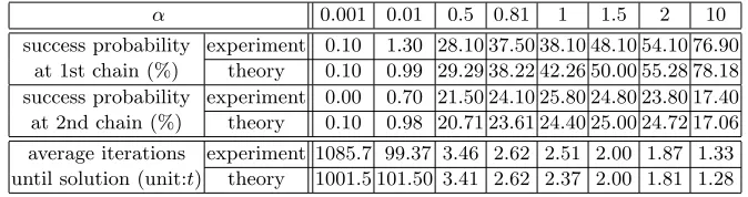
In Table 1, we compare our theory against experiment results under variations ofα. The success probability entries test the validity of Theorem 1 and the last two rows of the table test theT value as given by (6).
Table 2 shows a similar comparison under a fixedαand varyingmandtparameters. This table gives an indication of how well the relation (8) is observed, i.e., whether the increase in storage results in the predicted reduction of online time complexity.
5
Table 1.Online phase success probability and complexity for variousα(q: 42-bit prime,t= 214)
α 0.001 0.01 0.5 0.81 1 1.5 2 10
success probability experiment 0.10 1.30 28.10 37.50 38.10 48.10 54.10 76.90 at 1st chain (%) theory 0.10 0.99 29.29 38.22 42.26 50.00 55.28 78.18 success probability experiment 0.00 0.70 21.50 24.10 25.80 24.80 23.80 17.40 at 2nd chain (%) theory 0.10 0.98 20.71 23.61 24.40 25.00 24.72 17.06 average iterations experiment 1085.7 99.37 3.46 2.62 2.51 2.00 1.87 1.33 until solution (unit:t) theory 1001.5 101.50 3.41 2.62 2.37 2.00 1.81 1.28
Table 2.Online phase success probability and complexity for variousmandt(q: 42 bits prime,α= 0.81)
logt 8 11 14 17 20 theory
m 46121039 586463 12564 207 2 storage size (MB) 11806.986 150.135 3.216 0.053 0.001 success 1st chain 36.90 33.80 37.50 37.60 24.50 38.22 probability (%) 2nd chain 23.00 25.50 24.10 22.30 16.40 23.61 ave. iterations until solution (unit:t) 2.70 2.65 2.62 2.78 15.30 2.62
Test results given above are average values done over multiple table creations and multiple DLP target solving per created table. Each pre-computation table on experiments was created with a different random multiplier set for the 20-adding walk. All tests used 10 tables and 100 DLPs per table.
The implementation results support our theoretic analysis very well for a wide range of parameters. The only visible exception corresponds to when m is extremely small. In this case the expected DP chain length approaches the expected rho length of a random walk and thus too many chains are being discarded. Unlike the small m case, the results for large m follows the theory closely. This implies that the mPAP will work well even when extremely large storage is employed.
3.4 Parallelization
The pre-computation phase of themPAPcan trivially be parallelized. While pre-computation is certainly the computationally intensive part of the mPAP, there may be situations where the parallelization of the online phase is desired, possibly to reduce the wall-clock running time of the online algorithm further. Let us investigate this matter in this subsection.
Readers familiar with time-memory tradeoff techniques will have read the previous mate-rial withα≈1 in their minds, but one can confirm through a careful re-reading of all proofs that everything we wrote is true for even extremely smallα.
With Theorem 1 confirmed for small α, let us consider the parallel use of n processors at the online phase. We take parameters m and t such that mt2 = αnq, where α≈1. Then, based on Theorem 1, one can state that the probability of success at the first run of the online phase, i.e., after the nDP chains have been produced, is 1− 1
1+2α/n
n/2
can state
T1/n ≈
n
1 + 1
(1 +2nα)n2 −1
o
t
as the average time spent by each processor, until the DLP is solved. As before, we require M ≈m storage andP =mt pre-computation time.
Applying the equation mt2 = αnq, we can write the analogue to equation (7) as follows.
P T1/n ≈
α n
n
1 + 1
(1 +2nα)n2 −1
o
q. (9)
It is easy to check that 1 + eα1−1 ≤ 1 + (1+2α/n1)n/2−1 ≤1 + 1
√
1+2α−1, so that we can treat the term inclosed between the braces as an insignificant constant. Noting that n T1/n is the total online processing time, one can see that (9) is almost identical to (7). In other words, regardless of parallelization, with the same pre-computation effort, one needs the same total online processor time to solve a given DLP.
Analogue of (8) is as follows.
√
M T1/n≈
r
α n
n
1 + 1
(1 +2nα)n2 −1
o√
q (10)
and
P ≈
r
α n
√
Mpq. (11)
This says that withn-processor parallelization, one can achieve√ntimes online (wall-clock) time reduction and also an√nfactor reduction in pre-computation. A more practical view is to say that, by deciding to invest n-times more on the online processing power, one reduces the required cost of the pre-computation phase. Since the pre-computation is much more resource consuming than the online phase, in most situations, the less-than-linear speedup of the online phase will be justified by the reduction of pre-computation cost. In addition, if the parameters were such that the storage cost outweighed the processor cost, then one can surely justify the cost of additional processors.
3.5 Applying Tag Tracing Technique
In order to reduce the time for solving DLP over a finite field more, we consider applying tag tracing technique [7] to the mPAP. Since the mPAP consists of r-adding walk iterating function and DP collision detection method, the tag tracing technique can be applied to the
mPAP well. In this subsection, we confirm that the tag tracing technique works well in the
mPAP from experimental results.
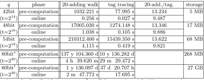
Test environment and implementation method of the mPAP were the same with Sec-tion 3.3. For the tag tracing technique, we stored all possible products of multipliers of 4-adding walk up to 40 steps using pre-computation with 54.9 MB and 36.951 seconds on average of all tests. Other parameters were set equal to experiments of Section 4.5 in [7] for fair comparison.
Table 3.Comparison of 20-adding walk and tag tracing (α= 0.81)
q phase 20-adding walk tag tracing 20-add./tag. storage 42bit pre-computation 1032.221 s 77.995 s 13.234 5 MB (t=214) online 0.256 s 0.027 s 9.487
48bit pre-computation 17005.030 s 1274.148 s 13.346 17 MB (t=216) online 1.038 s 0.105 s 9.886
54bit pre-computation 210312.400 s 15439.350 s 13.622 68 MB (t=218) online 4.115 s 0.419 s 9.821
80bit∗ pre-computation 137 y 104.360 d 10 y 136.282 d 268 MB (t=230) online 4 h 39.620 m 29 m 29.472 s
80bit† pre-computation 1 y 136.097 d 37 d 20.707 h 27 GB (t=230) online 2 m 47.772 s 17.695 s
estimated value (∗with 1 processor,†parallel processing with 100 processors)
Table 3 gives experimental results of applying 4-adding walk with tag tracing technique and 20 adding walk to themPAP. All results are average values done over 10 table creations and 100 DLP targets solving per created table. Each table was produced with a different random multipliers for use of differentr-adding walks.
We know that the use of 4-adding walk with the tag tracing technique is about 12 times faster than the use of 20-adding walk without the tag tracing technique from the result of [7] in our implementation environment. The last row in Table 3 shows that the tag tracing technique makes themPAP 9.487 – 13.622 times faster. This shows that applying tag tracing technique to themPAP works well.
Table 3 also provide the estimation time to solve a DLP using the parallelized mPAP with 100 processors.
4 Key Generation Time Estimation
In this section, we propose a parameter setup method of the MY-IBE scheme for achieving 280 security and efficiently generating a user’s private key. Then we estimate the key generation time on proposed parameters when applying the mPAP to KeyGen algorithm based on our complexity analysis and experimental results on small parameters.
4.1 Parameter Setup
In the MY-IBE scheme, the base groupG is taken to be a maximal cyclic subgroup of ZN∗
where N is a product of roughly same sized primes p, q such that p ≡ 3 (mod 4), q ≡ 1 (mod 4), and gcd(p−1, q−1) = 2. In order to obtain a secure MY-IBE scheme, as mentioned before, it is assumed that the CDH assumption in G holds and hence factoring N is to be hard.
Consider required conditions that N is hard to factor using known integer factorization algorithms within 280time complexity. First, N is to be at least 1024-bit integer (and hence both p, q are at least 512-bit primes) to endure against the number field sieve factorization algorithm [6]. Second, there are some factoring algorithms whose time complexity depends on the factorization ofp−1 and q−1. In case of the Pollard p−1 algorithm [22], it takes O(BlogN/logB) group operations to factorN wherep−1 andq−1 areB-smooth integers. Also, if factors ofp−1 orq−1 consist of one (logB)-bit prime and other (logB)/2-bit primes, then one can factorN within O(√B) operations using Brent’s method [5]. Hence one has to setp, qto be primes such that bothp−1 andq−1 are at least 280-smooth integers and have at least two prime factors of 80-bit or more.
However, the number of large prime factors ofp−1 and q−1 has a significant effect on the key generation time. Let us look into a process of solving a DLP in KeyGen algorithm of the MY-IBE scheme, which applies Pohlig-Hellman algorithm [21] with the mPAP. When an identity ID is given to KGC, he tries to compute the DL of H1(ID) to the base g. Since KGC knows the factorization ofN as trapdoor information, he can apply the mPAP or the Pollard rho algorithm to obtain H1(ID)ci’s to the base gci for allci’s whereci =p−1/pi or
q−1/qi, p−1 = Q`i=1pi, and q−1 = Q`i=1qi, i.e., he solves DLPs over subgroups of G,
whose order arepi’s andqi’s. Thereafter, he computes the DL ofH1(ID) to the baseg using
Chinese remainder theorem. In this process, large prime factors of p−1 and q−1 cause more key generation time or much memory size for themPAPto reduce key generation time. Hence, we recommend the use ofp, q such that both p, q are 512-bit primes and each p−1, q−1 has two 80-bit primes and other less than 40-bit primes.
4.2 Key Generation Time Estimation from Experimental Results
a maximal cyclic subgroup ofZN∗ whereN was an 1024-bit integer which was a product of
512-bit primesp, q and two prime factors ofp−1 andq−1 were (logB)-bit and other prime factors were less than (logB)/2-bit each. We utilized themPAPenhanced by the tag tracing technique [7] for solving DLPs on groups of four large prime factors and applied Pollard rho algorithm with 20-adding walk and DP collision detection method for solving DLPs on the other groups. Parameters for tag tracing technique were set equal to Section 3.5 and those for themPAP were set tot= 2(logB)/3,α= 0.81.
Table 4.Key generation time for variousB
securitypre-comp. pre-comp. online time storage level size time small factors large factors total
42 229.9 3 m 25 s 0.266 s 0.079 s 0.345 s 17 MB 48 233.9 54 m 45 s 0.495 s 0.310 s 0.805 s 68 MB
80∗ 251 13 y 231 d 3 m 12.605 s 2 h 52.578 m 2 h 55.788 m 270 MB
80† 251 49 d 19 h 1.926 s 1 m 43.547 s 1 m 45.473 s 27 GB
estimated value (∗with 1 processor,†parallel processing with 100 processors)
In Table 4, the third and fourth rows provide our experimental results of the key generation time corresponding to B, which are average values done over 10 table generations and 100 DLP targets solving per a created table. From these, when the difference between logB’s is d-bit, we are sure that the pre-computation time and the online-time for large prime factors are about 22d/3, 2d/3 times increased respectively and the online time for small prime factors is about 2d/4 times increased.
We estimate the pre-computation time and the online time for 280 security. Assume that we perform P = 251 pre-computation for four large prime factors and store 218 elements in each table. Then it takes about 13 years and 231 days for pre-computation with 270 MB storage. Since the pre-computation can be parallelized, one can generate the table in 49 days and 19 hours using 100 processors and 270 MB storage, in addition to the factors ofn, as the trapdoor information. When an instance of DLP is given, it can be solved in 2 hours and 56 minutes on one processor.
If, as described in Section 3.4, we decide to parallelize the online phase across 100 proces-sors while keeping the pre-computation at 251, the online phase reduces to one minute and 46 seconds with the use of 27 GB storage. Since this process is to be done by the key generation center to handle just key extractions, the presented pre-computation and online time may both be quite practical.
5 Conclusion
algo-rithm and gave more rigorous complexity analysis of themPAP. Also we discussed about the parallelization of themPAP and applying the tag tracing technique.
Finally, we gave the parameter setup method so that KGC efficiently solves a DLP and we estimated the key generation time on proposed parameter from our theoretical analysis and experimental results on small parameters.
References
1. L. M. Adleman. A subexponential algorithm for the discrete logarithm problem with applications to cryptography (abstract). InFOCS, pages 55–60. IEEE Computer Society, 1979.
2. S. Agrawal, D. Boneh, and X. Boyen. Efficient lattice (h)ibe in the standard model. In Advances in Cryptology - EUROCRYPT 2010, volume 6110 ofLNCS, pages 553–572. Springer, 2010.
3. D. Boneh and X. Boyen. Efficient selective-id secure identity-based encryption without random oracles. InAdvances in Cryptology - EUROCRYPT 2004, volume 3027 ofLNCS, pages 223–238. Springer, 2004. 4. D. Boneh and M. K. Franklin. Identity-based encryption from the weil pairing. In Advances in
Cryptology—CRYPTO 2001, volume 2139 ofLNCS, pages 213–229. Springer, 2001.
5. R. P. Brent. Some integer factorization algorithms using elliptic curves.CoRR, abs/1004.3366, 2010. 6. J. P. Buhler, H. W. Lenstra, and C. Pomerance. Factoring integers with the number field sieve. InThe
Development of the Number Field Sieve, volume 1554 ofLNCS, pages 50–94. Springer, 1993.
7. J. H. Cheon, J. Hong, and M. Kim. Speeding up the Pollard rho method on prime fields. InAdvances in Cryptology - ASIACRYPT 2008, volume 5350 ofLNCS, pages 471–488. Springer, 2008.
8. A. W. Dent and S. D. Galbraith. Hidden pairings and trapdoor ddh groups. InANTS, volume 4076 of
LNCS, pages 436–451. Springer, 2006.
9. Y. Desmedt and J.-J. Quisquater. Public-key systems based on the difficulty of tampering (is there a difference between des and rsa?). InAdvances in Cryptology – CRYPTO 86, volume 263 ofLNCS, pages 111–117. Springer, 1987.
10. C. Gentry. Practical identity-based encryption without random oracles. In Advances in Cryptology -EUROCRYPT 2006, volume 4004 ofLNCS, pages 445–464. Springer, 2006.
11. C. Gentry, C. Peikert, and V. Vaikuntanathan. Trapdoors for hard lattices and new cryptographic con-structions. InSTOC, pages 197–206. ACM, 2008.
12. Y. Hitchcock, P. Montague, G. Carter, and E. Dawson. The efficiency of solving multiple discrete logarithm problems and the implications for the security of fixed elliptic curves.International Journal of Information Security, 3:86–98, 2004.
13. J. Hong and S. Moon. A comparison of cryptanalytic tradeoff algorithms. Cryptology ePrint Archive, Report 2010/176, ver. 20110705:120703, 2011.
14. F. Kuhn and R. Struik. Random walks revisited: extensions of Pollard’s rho algorithm for computing multiple discrete logarithms. In S. Vaudenay and A. M. Youssef, editors,Selected Areas in Cryptography 2001, LNCS 2259, pages 212–229. Springer, 2001.
15. C. H. Lim and P. J. Lee. Modified maurer-yacobi’s scheme and its applications. In J. Seberry and Y. Zheng, editors,Advances in Cryptology - AUSCRYPT ’92, LNCS 718, pages 308–323. Springer, 1993. 16. U. M. Maurer and Y. Yacobi. Non-interactive public-key cryptography. In D. W. Davies, editor,Advances
in Cryptology - EUROCRYPT ’91, LNCS 547, pages 498–507. Springer, 1991.
17. U. M. Maurer and Y. Yacobi. A remark on a non-interactive public-key distribution system. In R. A. Rueppel, editor,Advances in Cryptology - EUROCRYPT ’92, LNCS 658, pages 458–460. Springer, 1993. 18. U. M. Maurer and Y. Yacobi. A non-interactive public-key distribution system. Designs, Codes and
Cryptography, 9:305–316, 1996.
19. Y. Murakami and M. Kasahara. Murakami-kasahara id-based key sharing scheme revisited — in comparison with maurer-yacobi schemes—. Cryptology ePrint Archive, Report 2005/306, 2005. http://eprint.iacr.org/.
21. S. C. Pohlig and M. E. Hellman. An improved algorithm for computing logarithms over GF(p) and its cryptographic significance. IEEE Transactions on Information Theory, 24:106–110, 1978.
22. J. M. Pollard. Theorems of factorization and primality testing.Cambridge Philosophical Society, 76:521– 528, 1974.
23. J. M. Pollard. A monte carlo methods for index computation mod p. Mathematics of Computation, 32:918–924, 1978.
24. J.-J. Quisquater and J.-P. Delescaille. How easy is collision search. New results and applications to DES. In G. Brassard, editor,Advances in Cryptology - CRYPTO, LNCS 435, pages 408–413. Springer, 1989. 25. J. Sattler and C.-P. Schnorr. Generating random walks in groups. Ann. Univ. Sci. Budapest. Sect.
Comput., 6:65–79, 1985.
26. A. Shamir. Identity-based cryptosystems and signature schemes. InAdvances in Cryptology—CRYPTO ’84, volume 196 ofLNCS, pages 47–53. Springer, 1984.
27. V. Shoup. NTL: A library for doing number theory ver. 5.5.http://www.shoup.net/ntl/, 2009.
28. H. Tanaka. A realization scheme for the identity-based cryptosystem. In Advances in Cryptology – CRYPTO 87, volume 293 ofLNCS, pages 340–349. Springer, 1988.
29. E. Teske. On random walks for Pollard’s rho method. Mathematics of Computation, 70(234):809–825, 2001.
30. E. Teske. An elliptic curve trapdoor system.Journal of Cryptology, 19(1):115–133, 2006.
31. S. Tsujii and T. Itoh. An id-based cryptosystem based on the discrete logarithm problem.Selected Areas in Communications, IEEE Journal on, 7(4):467 – 473, may 1989.
32. P. C. van Oorschot and M. J. Wiener. Parallel collision search with cryptanalytic applications. Journal of Cryptology, 12:1–28, 1999.
33. B. Waters. Efficient identity-based encryption without random oracles. In Advances in Cryptology -EUROCRYPT 2005, volume 3494 ofLNCS, pages 114–127. Springer, 2005.
34. B. Waters. Dual system encryption: Realizing fully secure ibe and hibe under simple assumptions. In